PowerPivot Example with SQL Server 2012

By: Daniel Calbimonte   |   Read Comments (1)   |   Related Tips: More > Microsoft Excel Integration

Problem

Sometimes we need to integrate different data sources to generate reports in SQL Server. We could use SSIS to integrate the data and use SSAS to generate reports. However, is there an easy way to generate some reports of data with millions of rows and integrating different data sources?  Check out this tip to learn more.

Solution

Yes - The answer is PowerPivot.  PowerPivot is an add-in for Microsoft Excel 2010 that allows you to import millions of rows of data from multiple data sources into a single Excel workbook.  With PowerPivot you can:

• Create relationships between heterogeneous data
• Create calculated columns and measures using formulas
• PivotTables
• PivotCharts

By building one or more of these items you can further analyze the data so that you can make appropriate business decisions.

But why Excel? Because everybody loves Excel and everybody knows how to use it. Learning the PowerPivot is then a straightforward task. You can import data from SQL Server, Oracle or other databases.  PowerPivot for Excel 2010 is used for data analysis, we can also transform large amounts of data into meaningful information really fast.  So let's dive in.

PowerPivot Requirements

To begin testing the PowerPivot we will need the following items:

• Excel 2010
• PowerPivot
• SQL Server 2012
• .Net Framework 4.5
• The AdventureWorks Database

Learning PowerPivot

Start by opening ‘Excel 2010’. A new PowerPivot Menu is added when you install PowerPivot as shown below:

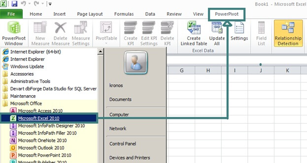
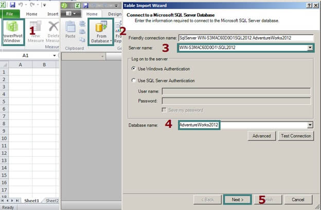
The steps to connect to the SQL Server database from 'Excel 2010' are the following:

1.- Click the Power Pivot Menu Option
2.- Click 'From Database' Icon
3.- Select the SQL Server instance
4.- Enter the Database name
5.- Press the 'Next' button

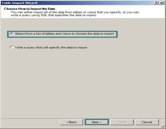
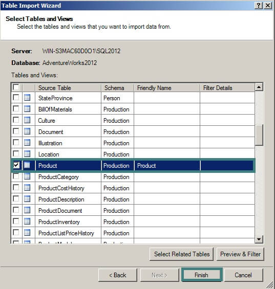
On the next screen, select the list of tables and views of data to import. You can select multiple tables or views or write a specific query.

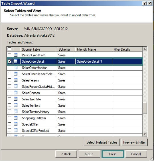
In our example, select the table 'Sales.OrderDetail' table and click the 'Finish' button.

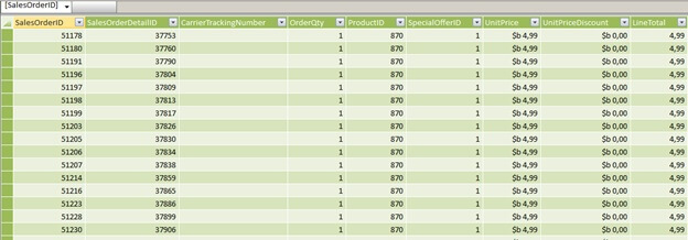
Now you have the SQL Server data in Excel. It is similar to the Pivot Tables, but faster.

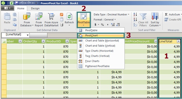
Build a PivotChart in Excel with PowerPivot

Below are the steps to generated a PivotChart in Excel with PowerPivot:

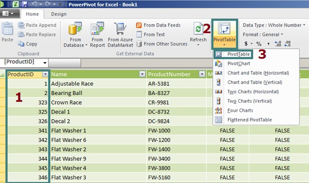
1.- Select the ‘Line Total’ column in Excel.
2.- Click the ‘PivotTable’ icon.
3.- Select the ‘Pivot Chart’ option.

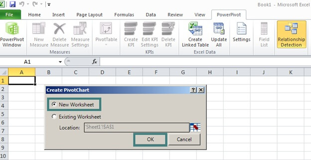
Select a 'New Worksheet' to display the chart and press OK.

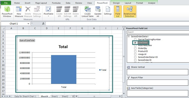
You can choose which column to graph from the PowerPivot Field List as shown below.

Building a PivotTable in PowerPivot

Now let's add more tables in PowerPivot by following the steps from above with the Table Import Wizard.  Let's add a new table to Excel. In this example we are adding the Production.Product table.

Now select the 'Product' table and the 'ProductID' column to create the relationship between SalesOrderDetail and Products tables.

1.- Select the column ProductID.
2.- Click the ‘PivotTable’ icon.
3.- Select ‘PivotTable’ from the menu.

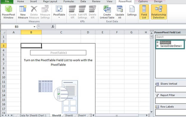
Now we have the 'Product' and 'SalesOrderDetail' tables to create queries from both tables as shown below.

Next Steps

• PowerPivot is an extremely flexible tool and a really easy to learn. You can create reports from multiple sources with millions of rows in a very rapid manner
• For more information, refer to these links:
  • Microsoft Excel Integration Tips
  • Introduction to PowerPivot for Excel and SQL Server

Last Update: 12/24/2012

About the author

Daniel is a Microsoft SQL Server MVP, Microsoft Certified Trainer and Microsoft Certified IT Professional.

View all my tips

We Recommend

• More Database Developer Tips...

Comments and Feedback:

Thursday, April 25, 2013 - 8:11:20 PM - Grace

Read The Tip

Hi Danial,    PowerPivot Example with SQL Server 2012 is nice article and helpfull, I have one doubt on PowerPivot refresh you may help me I have created PowerPivot data model and In DATA tab connection properties I selected Refresh for every and given 15 mins but data is not refreshing in PowerPivot data model, can you please let me know If I am missing anything to schedule data refresh for Power Pivot data model   Thank You, Grace

Post a Comment or Question

Keep it clean and stay on the subject or we may delete your comment.
Your email address is not published. Required fields are marked with an asterisk (*)

*Name

*Email

Notify for updates Signup for our newsletter

Comments *** NOTE *** - If you want to include code from SQL Server Management Studio (SSMS) in your post, please copy the code from SSMS and paste the code into a text editor like NotePad before copying the code below to remove the SSMS formatting.
*Enter Code

 

Sponsor Information

Find and fix SQL Server problems before they happen - SQL diagnostic manager now with predictive analysis! NEW! Top 5 hard-earned lessons of a DBA from Grant Fritchey & the DBA Team. Read it now Wish your SQL Servers could run wide open? Learn how the Edgewood SQL Server Consultants can make it happen. Secure column & whole database on all versions and editions of SQL Server with NetLib’s TDE Free SQL Server Learning - Lock Down SQL Server Security