SQL Server Analysis Services Period over Period Variance Analysis

By: Scott Murray   |   Comments (1)   |   Related: > Analysis Services Development

Problem

Often when working with OLAP cubes, the main "access" point will be an Excel pivot table. While utilizing OLAP cubes, end users will frequently want to compare two values from different periods in order to quantify some variance analysis processes; however the creation of calculations within OLAP based Excel pivot tables is not allowed.  What functionality is available to make these comparisons?

Solution

When pivot tables are created locally, calculated fields are easily created as part of the pivot table.  However, OLAP based pivot tables do not afford the ability to create these calculated values at the pivot table level. A few external tools exist, such as OLAP Pivot Table extensions available on CodePlex ( http://olappivottableextend.codeplex.com ); unfortunately most end users are not going to want to or have the ability to write the necessary MDX when working with this type of tool. Additionally, if you already have two measures to compare over the same time period, such as an actual versus budget, that calculation is easy mastered as both measures are readily available. Even so, your variance analysis must be part of the cube design; fortunately, using various functions including ParallelPeriod within calculated measure allows for easy variance analysis.

Variance Analysis-Period over Period

The initial step in completing the variance analysis is to first determine the measures which require variance analysis, and second determine upon which time dimension hierarchy or hierarchies, if multiples exists, to compare between periods, such as the most common year over year.  We will again use the AdventureWorks 2012 DataWarehouse and Cube for our examples.  In particular, we will use the Internet Sales Amount measure and the Calendar Date hierarchy for our examples.  Furthermore, we will use the ParallelPeriod function to determine the same period prior year value.  The ParallelPeriod function is described in detail in Ray Barley's tip: http://www.mssqltips.com/sqlservertip/2367/building-calculated-members-for-a-ssrs-report. The actual calculation to get the prior "parallel" period's value is displayed below with an explanation included thereafter.  

The statement is actually composed of two statements.  

First is the outer IIf function; this function handles the total value for the parallel period calculations.  Without this IIF statement, no totals would be displayed for the parallel period calculated measure. By checking to see if the CurrentMember is at level 0 (the base level or ordinal position for the selected date attribute), the total value only displays when the total is needed.

The second part of above statement contains the Parallel period function. This function requires 3 arguments.

• The first argument is the level expression; in basic terms, this argument will be the date member level that you are comparing.  For instance, it could be Calendar Year or Calendar Quarter or Calendar Month.  
• The second argument is the Index or number of lag periods to look back in order to find the ancestor value. For example if you specify a level of Calendar Year, and the index is 2, then the function would find the same period 2 years prior. Of course in accounting the most common lag is 1 year.  
• The last argument specifies what member expression is moved back the Index number of positions. In simpler terms, this argument is the starting member value upon which the level and index act upon.

In the example above, we use the Calendar Year attribute while finding the Internet Sales Amount for the same period 1 year prior using the Current Member of the Date.Calendar dimension hierarchy. Rolling all these items together, this calculated measure is added to the Adventure works cube as noted in the below example. Thus, first, Visual Studio 2010 (aka SQL Server Data Tools) will need to be started, and the Adventure Works SSAS database opened.  Next open the Adventure Works cube and switch to the Calculation tab.   

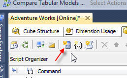
Now we define the calculated measure by clicking on the New Calculated Measure button.

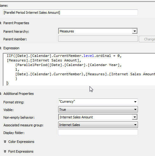
Next, enter a measure name; in this case Parallel Period Internet Sales Amount. Note that calculated measures with spaces in the name must be contained within brackets. Measures is selected for the Parent Hierarchy and the above expression is added to the expression box (this box contains the actual MDX expression).

Last, select the Format String of currency, Visible value of true, Non Empty Behavior of Internet Sales Amount, and last Associated Measure group of Internet Sales. The Non Empty Behavior field is important as it guides which calculations must be made for the calculated measure based on the measure you select; thus if the Non Empty Behavior measure value is Empty, this will guide SSAS to also mark the calculated measure as Empty which in turn improves performance by preventing this calculation to be made for all intersections of the selected dimensions.

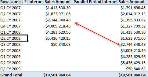
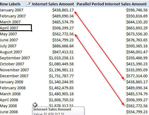
Enough digression on the inner workings of calculated values, but I would like to mention a couple of items about our calculated measure. First, since we are using the Date.Calendar hierarchy we can actually traverse any attribute of that hierarchy which falls under the attribute year noted in our level. Subsequently, if we drop Calendar Quarter, Internet Sales Amount and Parallel Period Internet Sales Amount on a pivot, we will see all Calendar Quarters along with the related Internet Sales Amount and the Internet Sales Amount for the Same Quarter one year prior. Since we used the CurrentMember in our member expression (third argument), we can actually switch out Calendar Quarter with Calendar Month, and now all months will be displayed along with the Internet Sales Amount plus the Parallel Period Internet Sales Amount from the same month 1 year prior.

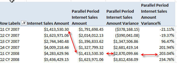
Both those scenarios are illustrated below.  

Now that the ParallelPeriod functionality is in place, we can continue developing our variance analysis. Our next calculation is a simple and which just determines the variance between the CurrentMember measures and the ParallelPeriod measure. Finally, we calculate the Variance % by dividing the variance amount by the ParallelPeriod value.  Both of these simple calculations are displayed below.

Initial examples of these calculations are displayed within the below Excel pivot table.

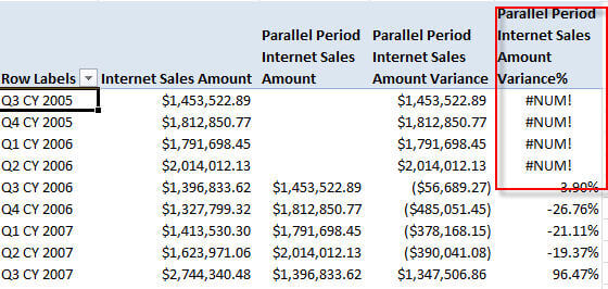
Of course a couple of problems surface with these calculations.  The calculation for the first period errors with a #NUM! error; this issue is more pronounced if we drill into quarters or months as noted in the second illustration displayed above. The problem is that there is no value for the prior parallel period. Let us address this issue by checking for the absence of a prior period value as described in the below MDX calculate measure.  

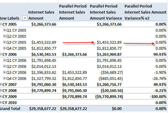
You may find it interesting that we are checking if our base calculation is equal to zero when the set or measures is actually empty, but SSAS treats many empty cells as zero. For an in depth reviewing on how SSAS treats empty measures or sets, please see the MSDN article in the Next Steps section at the end of this article. In the above example, we cover both possible instance by checking for a value of 0 or checking for an empty value using the IsEmpty MDX function. If either is true, then we set the Parallel Period Internet Sales Amount Variance% v2 measure to 0; otherwise we perform the variance calculation. The resulting pivot is displayed below. 

The above methods utilize a multi-tiered approach to solve our period over period variance analysis needs while at the same time providing flexibility in the use of variance time dimension attributes, such as quarters, months, and years. Just as with SQL, other MDX functions exist which could provide similar results to the parallel period calculation.  One such function is the Lag function which was covered in my tip on Lag / Lead functions in SSAS 2012, http://www.mssqltips.com/sqlservertip/2877/sql-server-analysis-serviceslead-lag-openingperiod-closingperiod-time-related-functions/. Furthermore, the Cousin function can also be used to complete period over period variance analysis. However, I find both these functions limit your flexibility if you want to navigate down the time dimension hierarchy as each requires a set level to traverse backwards (or forward in the Lead function's case).

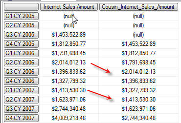
Below, an example of the cousin function is listed.  

Notice, how much more complicated the Cousin function is as compared to the ParallelPeriod function, and requires the use of the Ancestor and Lag functions also. The results of the above statement illustrated subsequently.

Conclusion

Variance analysis for SSAS OLAP cubes is not a simple matter of adding a calculated field to a pivot table. Planning along with the use of the ParallelPeriod MDX functions allows us to quickly create a variance infrastructure for a particular measure. Furthermore, by utilizing a date hierarchy in the Parallel Period function, we can easily traverse down the hierarchy for any attribute below the parallel period level noted in the function (i.e., parallel period based on Year can show either one year back per year, quarter, or month). Although, other methods exist, the parallel period method can be easily followed and applied to various measures.

Next Steps

• Sal De Loera's Alternate Method for adding Dynamic Time Calculation --http://saldeloera.wordpress.com/2013/02/07/ssrs-how-to-straightforward-method-to-pass-mdx-multi-select-parameters-to-mdx-datasets/
• MSDN--Working with Empty Values -- http://msdn.microsoft.com/en-us/library/ms145626.aspx.

About the author

Scott Murray has a passion for crafting BI Solutions with SharePoint, SSAS, OLAP and SSRS.

This author pledges the content of this article is based on professional experience and not AI generated.

View all my tips