By: Scott Murray | Comments | Related: > Analysis Services Measure Groups
Problem
I have several fact tables at varying levels of granularity for a SQL Server Analysis Services (SSAS) cube; how can I handle this situation and still use just a single cube?
Solution
The level of granularity you use for a cube and its measure groups is probably one of the most important initial considerations that must be made when starting a SSAS data warehouse project. Granularity levels define the lowest level of detail that will be conveyed in a cube; of course, you can create drill through actions that can implement database queries to obtain lower levels of detail (see https://www.mssqltips.com/sqlservertip/3168/excel-actions-and-drill-down-for-sql-server-analysis-services/). Furthermore, SSAS actually provides direct methods of utilizing the same cube for reporting on granularity levels that are higher than the lowest level of detail, just not any levels that are lower. This situation is often seen when you have varying fact tables that will be included in a cube. A few examples of these situations include: 1) having sales details at the day level, but budget data for the same sales at the weekly or monthly level 2) having sales at a product detail level, but having sales commission targets at the product category level 3) having promotions only be offered at the country level and not at the individual state and province levels. For these examples, generally the data values are only accounted for at the rolled up level as generating the data at the lowest level of detail is too cumbersome. So how can we handle these situations? Fortunately, SSAS allows us to set up varying dimension usage based on individual measure groups. Thus, to adjust upward the level of granularity, we must adjust how we define each attribute usage relationship.
We will use the Adventure Works databases as the basis for our SSAS example. The 2014 versions of the regular and data warehouse databases, along with the SSAS cube database backups are available on Codeplex: https://msftdbprodsamples.codeplex.com/releases/view/125550. Once you download and install the SQL Server and SSAS databases, we will subsequently use SQL Server Data Tools for Business Intelligence (SSDT-BI) for Visual Studio 2013 to work through the SSAS granularity levels. You can download SSDT-BI from: http://www.microsoft.com/en-us/download/details.aspx?id=42313.
Defining Granularity in a Fact Table
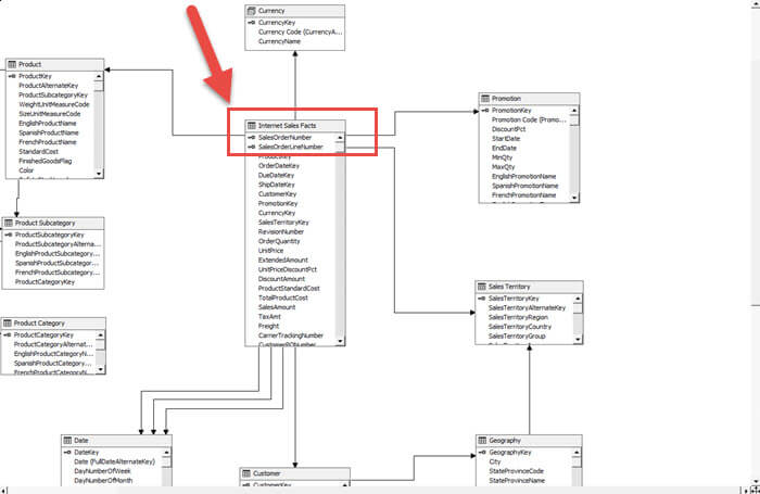
When you define granularity, you always need to start from the lowest level and work your way up; of course you can create actions to drill into lower levels, but those actions will take you outside of your cube browser, for instance outside of an Excel Pivot Table. For our example we will use the Adventure Works DW SSAS cube. Specifically, let us look at the Internet Sales Fact table in the data source view; this table uses SalesOrderNumber and SalesOrderLineNumber as the keys. This setup means that the combination of SalesOrderNumber and SalesOrderLineNumber are the lowest level of granularity. In its simplest form, surrounding this fact table are various dimensions ( or lookup tables ) for product, promotion, customers, date, and sales territory, among others.
However, say that total sales budget figures have been established for each employee per each month. As shown in the below screen print, the budget figures are not concerned with breakouts by product, promotion, currency or customer. Plus the data is based on monthly figures and not daily figures.
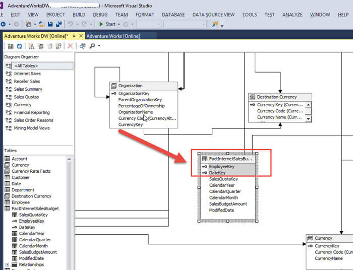
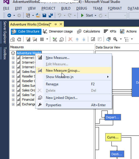
Of course, we could create a separate cube for just this fact dataset and its related dimensions. However, it is also very convenient and in many cases more efficient to just create a separate measure group within our existing SSAS cube, with the understanding that this data will be rolled farther up the granularity chain. Thus, after adding the FactInternetSalesBudget table to our data source view, we need to first add a new Measure Group, for the Sales Budget Amount in our example table. The first step in adding the measure group is shown below.
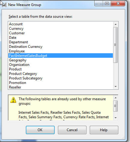
Next we select the FactInternetSalesBudget table as the basis for our new measure group.
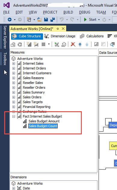
Last, SSAS creates the Fact Internet Sales Budget measure group, and adds a default set of measures. As shown below, we clean up the names to be more descriptive. The final result is a new measure group, Fact Internet Sales Budget, with two measures, Sales Budget Amount and Sales Budget Count.
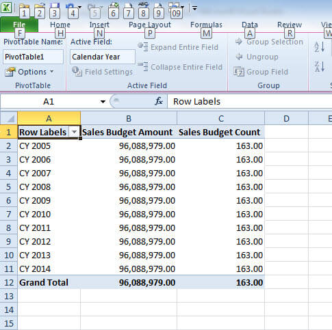
Now that our measure group is created, we need to reprocess the cube for the measure group additions to take effect (see https://www.mssqltips.com/sqlservertip/2203/processing-an-analysis-services-cube-using-sql-server-management-studio/ or https://www.mssqltips.com/sqlservertip/2936/sql-server-analysis-services-partition-maintenance-and-processing/). Wow, that was easy right; unfortunately the results are less than spectacular as illustrated next. We have the total amounts for every row.
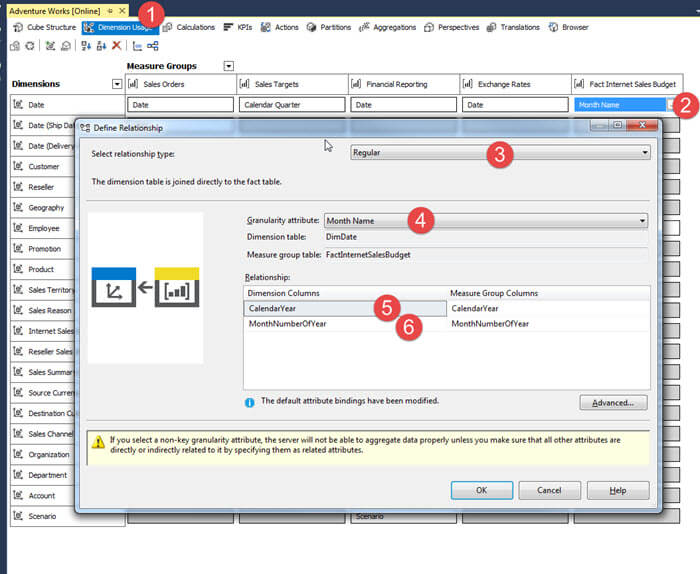
To fix this situation we need to complete several steps, the first of which is to update the dimension usage tab with the proper relationship for our measure group, step 1 in the below screen print. Next, step 2, we need to scroll to the Fact Internet Sales Budget measure group and click on the dash on the Date dimension box. Next on the Define Relationship window, we select a Regular relationship type, which is step 3. In step 4 we select the Month Name as the level of granularity. This field specifies the lowest level of granularity for this measure group. Finally in steps 5 and 6 we must specify the relationship of CalendarYear and MonthNumberofYear for the relationship joins for the date dimension (and not using the data key).
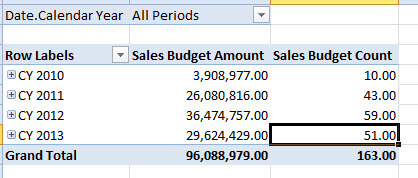
Now, refreshing the pivot table shows the correct breakout for our
date dimension; as seen in the below screen print, no duplicates are
shown.
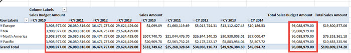
Unfortunately, when we add a non related dimension to the pivot, the duplicates return. Remember, the sales budget data is not broken out by sales territory region for this example.
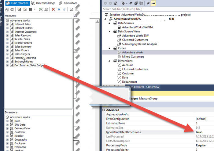
To alleviate these duplicate values, we need to adjust the measure group's IgnoreUnrelatedDimensions property to false.
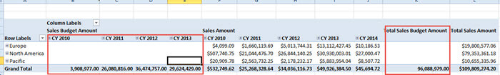
By adjusting this property, now we only see the data at the total level, as shown next. Also, notice how the Sales Amount ( from the Internet Sales measure group) shows the appropriate level of detail. I believe this setup is preferable to having the data shown with duplicates.
Conclusion
Contrary to popular belief, SSAS does provide a method for showing different levels of granularity within a cube, as long as the level is higher than the base or lowest granularity level. In order to complete this process, a separate measure group must be created for the fact table which will be at the higher level. Once the measure group is created, then dimensions can first be joined to the measure group at varying levels; for example instead of joining a date dimension at the date level; it could be joined at the month / year level. Furthermore, not all dimensions must be included or "joined" to a measure group. In those cases to prevent duplicates from showing within the cube browsers, it is recommended that the IgnoreUnrelatedDimensions measure group setting be set to False. By combining all these techniques, cube designers can keep all the facts and dimensions in a single cube.
Next Steps
- Review all the SSAS Measure Group Tips - https://www.mssqltips.com/sql-server-tip-category/153/analysis-services-measure-groups/


About the author
 Scott Murray has a passion for crafting BI Solutions with SharePoint, SSAS, OLAP and SSRS.
This author pledges the content of this article is based on professional experience and not AI generated.
View all my tips