By: Maria Zakourdaev | Comments | Related: > Python
Problem
When it comes to data-driven research, presenting the results is a complicated task. It is convenient to have an initial dataset handy, if anyone asks to re-run the computations or wants to interact with the data. Reproducibility across a number of fields is a tough task and there aren’t too many tools that can help. It’s easy to show numbers in Excel or in Power Point, but in many use cases, the context and the pathway to the results is lost.
Solution
What is the Jupyter Notebooks?
Jupyter Notebooks is a great tool that is becoming more and more popular these days. Jupyter Notebook combines live code execution with textual comments, equations and graphical visualizations. It helps you to follow and understand how the researcher got to his conclusions. The audience can play with the data set either during the presentation or later on. Some people say that Project Jupyter is a revolution in the data exploration world just like the discovery of Jupiter's moons was a revolution in astronomy.
Project Jupyter history
Project Jupyter was started as an academic challenge. Since 2011 it’s an open-sourced product and can be easily installed using Python Anaconda distribution that includes iPython kernel, Jupyter server and most popular libraries. It supports over 100 programming languages and additional kernels, but Python is the most popular. There are more than 2 million notebooks published on GitHub these days, lots of customizations and addons. Jupyter got its name from three programming languages, Julia, Python and R.
Jupyter Notebooks can be deployed on your laptop or on any cloud server. Moreover, all cloud service providers have Jupyter-as-a-service, for instance Microsoft Azure Notebooks, Google CoLab or AWS SageMaker and there is a Binder executable service which allows you to execute and play with any notebook stored in GitHub without installing anything on your laptop.
If you are new to Jupyter Notebooks, I suggest you to go to Microsoft Azure Notebook by Buck Woody where you can learn about the Jupyter Notebook power and after playing with the notebook, come back to this tip.
In this tip I will show you how Jupyter Notebook helps you to make a presentation based on the data research. After having the initial result set into the dataframe variables, you will not need a connection to the database and can rerun any computation that your audience will demand. You can visualize the results with one line of the code and I am sure that your audience will be impressed.
Built-in iPython magic
iPython kernel has built-in magic commands. Those commands use symbol %, which is not a valid unary operator in Python and can be used only in combination with a magic command. There are many magic commands for different purposes.
In this tip we will talk about %sql magic which can be used for interactive data analysis using our favorite language: SQL. We can query any database system; in this tip I will use SQL Server.
Environment preparation
To play with the below examples, you can either use any cloud Jupyter service, prepare your own environment or you can launch it in the server-less executable environment Binder.
Full Jupyter Notebook is available here on GitHub. If you are setting up your own environment, to query SQL Server you will need the MSSQL ODBC driver installation and I have added the below code to the /etc/odbcinst.ini file:
[sqlsrv]
Description=Microsoft ODBC Driver 17 for SQL Server
Driver=/opt/microsoft/msodbcsql17/lib64/libmsodbcsql-17.3.so.1.1
UsageCount=1
If you already have the Python distro, make sure you have the below packages installed:
Pip3 install jupyter
pip3 install ipython-sql
pip3 install sqlalchemy
Pip3 install pandas
Pip3 install matplotlib
Pip3 install numpy
%SQL magic Jupyter Notebook:
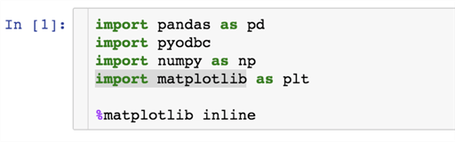
First, we are loading iPython sql extension and python libraries that we will use in this Notebook
%load_ext sql
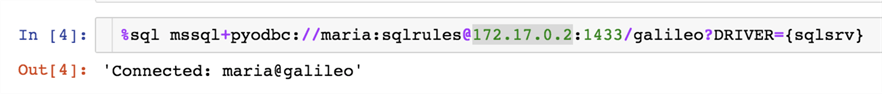
Now we will connect to our database. I am using local docker here, you can connect to your SQL Server instance using SQL Alchemy format (Object Relational Mapper for Python).
The connection string format 'mssql+pyodbc://user:password@server/database?DRIVER={enty in /etc/odbcinst.ini}'
In order to create simple objects used in this demo you can run the following statements:
create table products( productid int, productname varchar(256));
create table orders( productid int, customerid int, quantity int );
create table customers( customerid int, firstname varchar(256), lastname varchar(256));

insert into customers
select object_id+200,'firstname' + cast(object_id+200 as varchar),'lastname' + cast(object_id+200 as varchar) from sys.objects

insert into products
select object_id+200,'product_' + cast(object_id+200 as varchar) from sys.objects
insert into orders
select productid, customerid, (ABS(CHECKSUM(NewId())) % 14 ) * 10 from products,customers
Querying
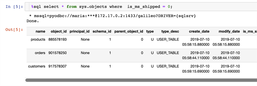
We will start with the simple query.
If your query is short, you can use one-line of code:
%sql select * from sys.objects where is_ms_shipped = 0;
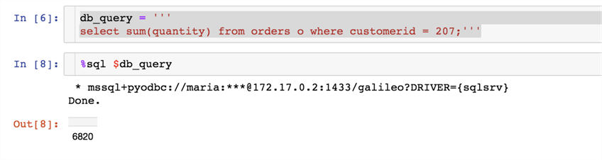
If the query spans several lines, you can put the query into a variable and execute it:
db_query = '''
select sum(quantity) from orders o where customerid = 207;'''
Using variables
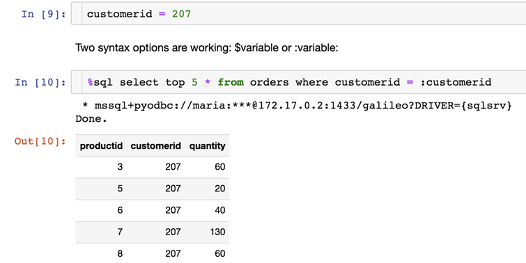
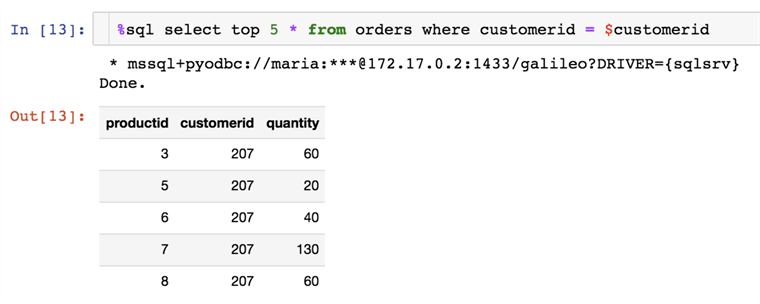
For data exploration and presentation, its handy to load the data from the database into the variable.
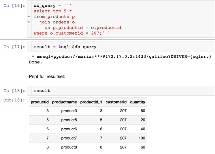
db_query = '''
select top 5 *
from products p
  join orders o
    on p.productid = o.productid
where o.customerid = 207;'''

result = %sql $db_query
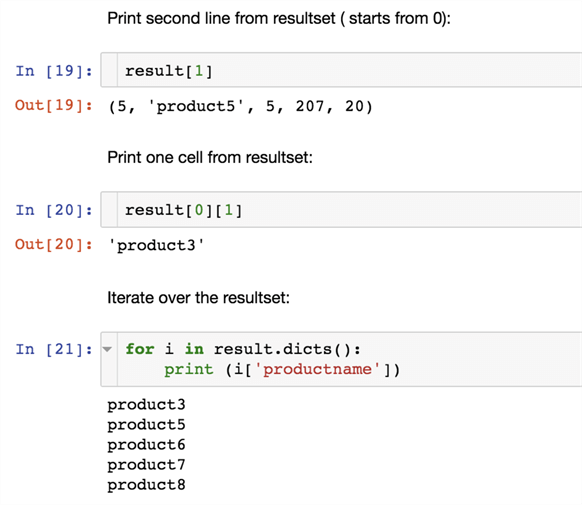
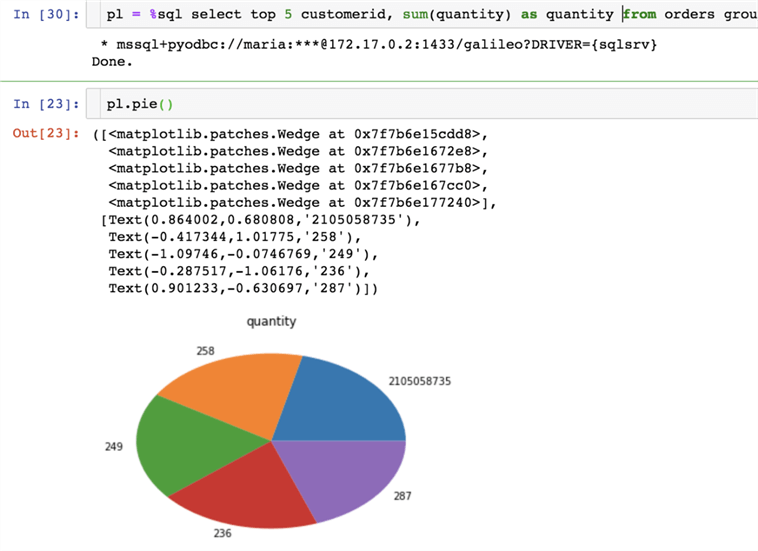
Look, how easy is to visualize the result using the matplot library:
pl = %sql select top 5 customerid, sum(quantity) as quantity from orders group by customerid order by sum(quantity) desc;
pl.pie()
Dataset generation
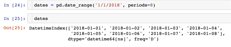
In this example we will use pandas.date_range() - one of the general functions in Pandas which is used to return a fixed frequency.
We will generate a list of 8 dates starting with 1/1/2018
dates = pd.date_range('1/1/2018', periods=8)
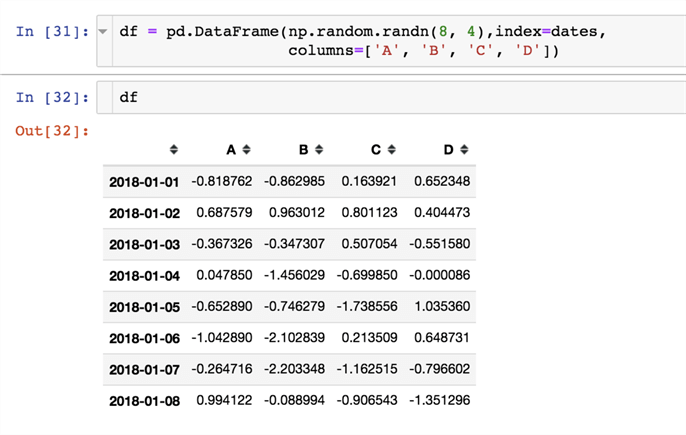
numpy.random.randn(d0, d1, …, dn) : creates an array of specified shape and fills it with random values.
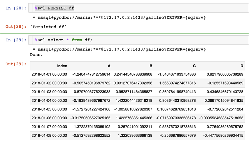
Persisting dataset into the database
The PERSIST command will create a table in the database to which we are connected, the table name will be the same as dataframe variable.
%sql PERSIST df
%sql select * from df;
In this tip we learned how to use the power of Python and %sql magic command to query the database and present the results. Since you have the initial result set inside dataframe variables, you will not need a connection to the database and can rerun any computation that your audience needs. You can visualize the results with one line of the code and I am sure your audience will be impressed.
Next Steps
- Jupyter Project home: https://jupyter.org/
- Jupyter Notebook Introduction: https://realpython.com/jupyter-notebook-introduction/
- Binder – making your notebooks interactive: https://ovh.mybinder.org/
- You can run this notebook using this link in Binder, connect to your database and play with the above mentioned commands.


About the author
 Maria Zakourdaev has been working with SQL Server for more than 20 years. She is also managing other database technologies such as MySQL, PostgreSQL, Redis, RedShift, CouchBase and ElasticSearch.
This author pledges the content of this article is based on professional experience and not AI generated.
View all my tips