Using Simple Linear Regression to Make Predictions

By: Nai Biao Zhou   |   Comments (1)   |   Related: More > R Language

Problem

Regression analysis may be one of the most widely used statistical techniques for studying relationships between variables [1]. We use simple linear regression to analyze the impact of a numeric variable (i.e., the predictor) on another numeric variable (i.e., the response variable) [2]. For example, managers at a call center want to know how the number of orders that resulted from calls relates to the number of phone calls received. Many software packages offer expertise in regression analysis, such as Microsoft Excel, R, and Python. Following the tutorial [3], anyone who knows Microsoft Excel basics can build a simple linear regression model. However, to interpret the regression outputs and assess the model's usefulness, we need to learn regression analysis. As Box [4] said, "all models are wrong, but some are useful." To be capable of discovering useful models and make plausible predictions, we should have an appreciation of both regression analysis theory and domain-specific knowledge. IT professionals are experts in learning and using software packages. All of a sudden, business users ask them to perform a regression analysis. IT professionals whose mathematical background does not include a regression analysis study want to gain the skills to discover plausible models, interpret regression outputs, and make inferences.

Solution

Many software packages provide comprehensive features for fitting regression models to a data set. In addition to Porterfield's MS Excel tutorial [3], Chauhan wrote a beginner's guide [5] that built regression models by employing Python. The blog [6], posted by Martin, explained using R programming to find a mathematical equation that predicts cherry tree volume from metrics that are practical to measure. As far as regression analysis is concerned, understanding regression analysis techniques strongly outweighs operating these regression tools. This tip aims to introduce just enough regression analysis; then, IT professionals who have limited exposure to regression analysis, can start to investigate the relationship between numeric variables.

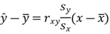
Aristotle said that every effect has a specific cause or causes [7]. In the cause-and-effect relationship analysis, the reason denoted by X is called the predictor variable, and the result denoted by Y is called the response variable. Such a relationship implies that we can predict the value of the response variable Y in terms of a set of predictor variables X. These variables have other names. Predictor variables are also called independent variables, regressors, controlled variables, explanatory variables, or input variables. Response variables are called regressands, dependent variables, explained variables, or output variables. However, a regression model does not imply a cause-and-effect relationship between the variables.

A simple linear regression analysis studies a straight-line relationship between a single response variable and a single predictor variable. In the business world, a single response variable may depend on two or more predictor variables. Linear regression analysis in a multi-dimensional space is called multiple linear regression analysis. I expect this tip to lay the groundwork for performing multiple linear regression analysis by exploring a simple linear regression analysis.

To estimate the effect of an increase in the number of calls during a work shift on the number of orders that resulted from these calls, I adopt the six-step procedure [8] to perform the simple regression analysis:

1. Hypothesize a form of the model;
2. Collect the sample data;
3. Estimate unknown parameters in the model;
4. Perform residual analysis;
5. Assess the usefulness of the model;
6. Apply the model for predictions;

We may be excited about making predictions through linear regression analysis. However, it is rarely possible to predict a single value of the response variable precisely in terms of the predictor variable. Knowing averages (or expected values) of the response variable and confidence intervals of the predictions is sufficient in most situations. For example, we may not accurately predict how many orders the call center obtains when the call center receives 120 phone calls during a particular shift. However, following this six-step procedure, we can predict the average number of customer orders received during a work shift in terms of the number of phone calls.

I designed this tip to assist IT professionals who already know some statistics concepts: mean, variance, statistical significance, standard deviation, normal distribution, correlation, covariance, parameter estimation, and hypothesis testing. My other tips [9,10,11,12,13,14,15] have already covered these concepts.

This tip consists of two parts. The first part focuses on using an R program to find a linear regression equation for predicting the number of orders in a work shift from the number of calls during the shift. We randomly choose 35 work shifts from the call center's data warehouse and then use the linear model function in R, i.e., lm(), to find the least-squares estimates.

The second part is devoted to the simple linear regression analysis. There are six essential steps involved in the regression analysis. For hypothesizing a form of the model, Section 2.1 introduces an approach to discover the response variable and the predictor. In Section 2.2, we explore two sample data types for regression and suggest a rule of thumb to determine the sample size. Next, in Section 2.3, we use the least-squares method to compute the estimator of model parameters.  Section 2.4 makes four standard model assumptions. The inferences from linear regression are more accurate when the residuals have a normal distribution. Then, in Section 2.5, we test whether the predictor variable contributes information for predicting the response variable. The last section in part 2 uses the regression function to make predictions.

Regression analysis is an iterative procedure [1]. We fit a hypothesized regression model to sample data. Then we perform model adequacy checking. If we do not satisfy the hypothesized model, we come back to step one and choose other model forms.

The sample data are from the Microsoft sample data warehouse AdventureWorksDW2017[16], which contains operational data recorded by a fictitious call center. The call center divides a working day into four shifts: AM, PM1, PM2, and Midnight. The database table "FactCallCenter" includes two columns "Calls" and "Orders." Data in the Calls column represent the number of calls received during a shift. The Orders column contains the number of orders that resulted from telephone conversations in that duty period. The table has 120 rows; however, the table could have a significant amount of data in practice since it stores data for everyday operations. I tested code used in this tip with Microsoft R Client 3.5.3 on Windows 10 Home 10.0 <X64>. The DBMS is Microsoft SQL Server 2017 Enterprise Edition (64-bit).

1 – Using R to Find a Linear Regression Equation for Predicting

Call center managers in Adventure Works Cycles [16] want to know the form of relationship between the number of orders that customers placed in a shift to the number of calls received during the shift. It is reasonable to ask whether the number of orders depends on the number of calls received; therefore, the number of orders is the response variable Y. The number of phone calls is the predictor X. To use the simple linear regression model, we assume the regression function is linear:

where denotes the error term, the intercept and the slope are unknown parameters.

In practice, we cannot measure X and Y in the entire population; therefore, the parameters and are unknown. We estimate them using sample data. We use and to denote estimators of and , respectively; therefore, the following equation represents a straight line that best fits the sample data:

where is an estimator of the mean value of Y for a given value x.

Several factors determine the sample size n; as a rule of thumb, the sample size should not be less than ten times the number of estimated parameters in the model [8]. The following R code simulates the sampling process to select 35 shifts from the database. We then use the function lm() in R to find the fitted simple linear regression model.

# Load Package RODBC
library(RODBC)

# Define the query
sql.query <-'SELECT[Calls], [Orders] FROM[AdventureWorksDW2017].[dbo].[FactCallCenter]'

# Open connection to the ODBC database
channel <- odbcDriverConnect('driver={SQL Server};server=.;database=AdventureWorksDW2017;trusted_connection=true')

# Read the data into a data frame
data.frame.orders <- sqlQuery(channel,sql.query)

# Close connection
odbcClose(channel)

# Set the seed of R random number generator
set.seed(2020)

# Draw 35 sampling units randomly from the population
sample.orders <- data.frame.orders[sample(nrow(data.frame.orders), 35, replace = FALSE),]

# Obtain and print regression model for the simple linear regression
model <- lm(Orders ~ Calls, data = sample.orders)
print(summary(model))

## Generates diagnostic plots for evaluating the fit of a model
## Set the plotting area into a 2*2 array
#par(mfrow = c(2, 2))
#plot(model)
## Restore original settings
#par(mfrow = c(1, 1))
# The attach function allows to access variables of a data.frame without calling the data.frame.
attach(sample.orders)

# Create a scatterplot.
plot(Calls, Orders, xlab ="The number of orders that resulted from calls",
                    ylab ="The number of calls received during the shift")

# Add the fitted line.
abline(model, lty ="dashed")

# Remove the attachment of the data.frame,
detach(sample.orders)

The R program plotted a scatter diagram to examine the relationship between the number of orders and the number of calls. The scatter diagram shown in Figure 1 implies a positive linear association. As the number of calls received during a shift increases, the number of orders results from calls increases. Such a linear pattern allows us to use a straight line to represent the relationship; therefore, a simple linear regression model is appropriate for the regression analysis. My other tip [10] introduces how to compute the correlation coefficient, which measures the strength and direction of the relationship between two variables. We use a term bivariate to name this type of two-dimensional data. We can perform a simple regression analysis when the correlation within the bivariate data is at least moderately strong.

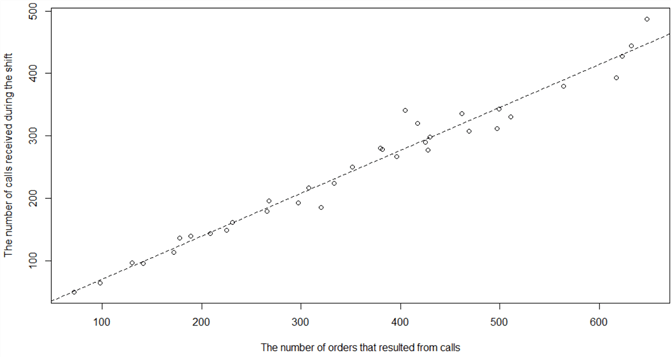
Figure 1 The Scatter Diagram with the Regression Line

The regression model outputs shown in Figure 2 reveal that the intercept's estimator is 2.07, and the estimator of the slop is 0.69. The least-square regression line intercept 2.07 estimates the mean number of orders when the call center receives 0 phone calls. Since we do not have data collected at or near this data point, the interpretation of the intercept is meaningless. It is noteworthy that making predictions using X values that fall outside the sample data range is not practical. The interpretation of the least-squares regression line slope 0.69 (69/100) is that the mean number of orders will increase by 69 on average for every 100 increase in the number of calls received.

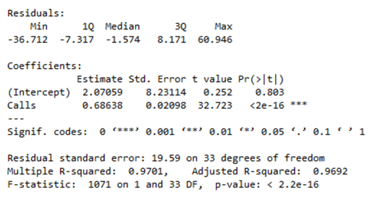
Figure 2 Regression Model Outputs

The following equation represents the fitted simple linear regression model, and we can use this line to predict the number of orders in a shift. To make predictions, we plug the number of calls received into the equation and solve for customer orders.

For example, the call center receives 120 calls during a shift. Using the regression equation, we find the average number of orders placed in the period is (2.07 + 120 X 0.69) = 84.87. We can predict that the number of orders placed in the period is probably about 85 when the call center receives 120 calls during the shift.

We estimated these two model parameters based on sample data. These estimates typically change when we select other samples. The totality of methods covered in this section is more like a curve-fitting exercise than simple linear regression analysis. To complete the regression analysis, we should make inferences about model parameters. The inference procedure involves three main elements: point estimation, hypothesis testing, and construction of confidence sets.

2 – Simple Linear Regression Analysis

Although we already know how to conduct linear regression analysis using software packages, we should understand the fundamental statistical concepts behind linear regression. Without learning some math and statistics, we are in a danger zone, illustrated in Figure 3. As Conway [17] pointed out, people in this zone can achieve a legitimate analysis without understanding how they got there or what they have created. These people can build a model that seems to work as expected, but the model can fail and therefore produce misleading results.

Figure 3 Drew Conway's Venn Diagram of Data Science [17]

This exercise adopts a six-step procedure [8] to walk through simple linear regression analysis systematically and logically. This procedure covers critical steps in regression analysis, including hypothesizing a form of the model, collecting the sample data for regression, estimating unknown parameters in the model, performing residual analysis, assessing the model's usefulness, and making predictions.

2.1 Hypothesize a Form of the Model

Regression is a method for studying the relationship between a response variable and a set of predictor variables. We can describe the relationship through a regression function [18]. The regression functions could be in many forms that represent different types of regression models. Frost [19] explored some common types of regression analyses, and we can choose one that fits our data. As we are dealing only with the simple linear regression model in this tip, the predictor variable is one-dimensional:

We may consider this equation to be a population regression model. The error term can arise in various ways:  randomness, measurement error, lack of knowledge of other important influences, etc. Since the simple linear regression analysis involves two variables, we must identify the response variable X and the predictor variable Y. A practical approach is to evaluate the following two claims and select the more reasonable one [20]:

1.     The first variable depends on the second variable.
2.     The second variable depends on the first variable.

When we examine the relationship between the number of calls received during a shift and the number of orders resulted from phone conversations, it is reasonable to say that the number of customer orders depends on the number of phone calls. In this exercise, the number of phone calls is the predictor variable, denoted by X, and the number of orders is the response variable, denoted by Y.

2.2 Collect the Sample Data

Observational data and experimental data are two types of data for regression analysis. If we have no control over the values of predictor variables, the data we collect for regression are observational. For example, the call center cannot pre-determine the number of calls received during a shift; therefore, the sample data used in Section 1 are observational. In experiments, researchers can plan predictor variables to generate experimental data. For example, we want to discover the effect of the running speed on the heart rate. We run on a treadmill with several equally spaced velocities for this experiment, then monitor heart rates corresponding to each speed. Book [8] reminds us that regression analysis based on observational data has more limitations than experimental data analysis. Besides, using historical data also involves some risks [1].

Determination of sample size is one of the most critical steps in the sampling process. My other tip [12] lists two criteria to determine the sample size, i.e., the precision level and the confidence level. The regression analysis also needs to estimate additional model parameters.  Therefore, in regression analysis, the sample size should be large enough so that these parameters are both estimable and testable.

As a rule of thumb, a sample should be at least ten times bigger than the number of additional parameters in the model [8]. For the simple regression analysis, excluding the intercept, the model has one unknown parameter (i.e., the slope); therefore, the sample size should be at least ten. Taking the precision level and the confidence level into considerations, the sample size for simple regression analysis should be at least 30. In this tip, we randomly select 35 sampling units, shown in Table 1:

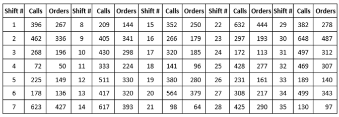
Table 1 Sample Data for Simple Regression Analysis

When a sample is ready, we should visualize and examine the data with a scatter diagram. If the visual aid does not suggest there is at least somewhat of a linear relationship, the hypothesized form may not be appropriate for the data. We may need to apply other regression techniques, for example, transformations. Figure 4 portrays the sample data in Table 1.  The scatter diagram suggests a positive linear association, and the correlation in the bivariate data is moderately strong. As the number of calls received during a shift increases, the number of orders results from calls tends to increase. Such a linear pattern allows us to use a straight line to represent the relationship; therefore, a simple linear regression model is appropriate for the regression analysis.

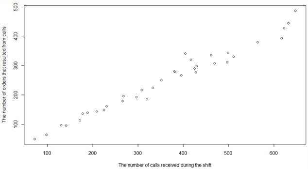
Figure 4 The Scatter Diagram for Sample Data in Table 1

2.3 Estimate Unknown Parameters in the Model

We have obtained the hypothesized form in Section 2.1, and we have collected sample data in Section 2.2. Now we are ready to estimate these two unknown parameters in the model using the method of least squares. To evaluate the simple linear regression model, we compare the model to a baseline model with only a response variable. The baseline model also serves as a null hypothesis model for testing whether the predictor's effect on the response variable is significant [2].

2.3.1, Horizontal Line Regression

Assuming we only record the number of customer orders resulting from calls, we randomly select 35 shifts, as shown in Table 2. We want to establish a model that predicts the number of customer orders in a work shift.

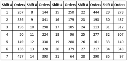
Table 2 Sample Data for Horizontal Line Regression Analysis

When we want to predict the number of orders for shifts using only the response variable, a horizontal line regression model fits this situation. Since there is no other information available, we always make the same prediction for any work shift. The response variable's mean is the sum of a constant, denoted by μ, and a random error component, indicated by ε:

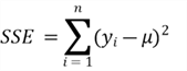
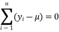
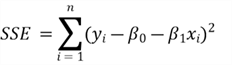
To find a straight line that best fits the sample data, we expect the prediction errors should be as small as possible. Figure 5 illustrates the errors of prediction (or residuals). Since a prediction error might have negative values, we use the sum of squares of the errors (SSE) to measure how well the line fits the data. The SSE also emphasizes those points that are far away from the horizontal line.

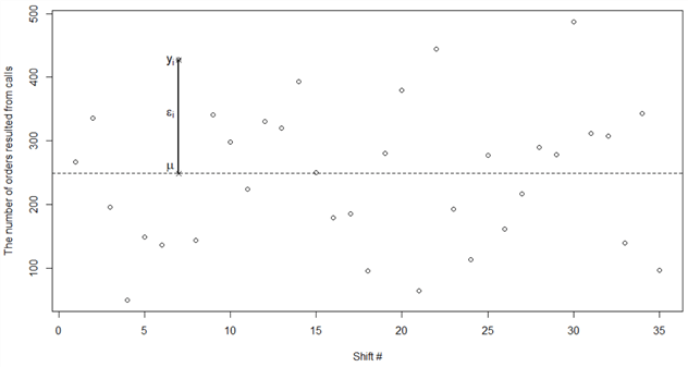
Figure 5 Horizontal Line Regression

If we move the horizontal line up and down, the SSE changes accordingly. We want to find a horizontal line that makes SSE a minimum. We call this line the least-squares line, regression line, or least-squares prediction equation [8]. We use a mathematical procedure, namely the least-squares method, to find the horizontal line regression. To minimize the SSE, we use the standard calculus procedure to set the derivative of SSE to zero and solve for µ:

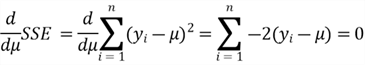
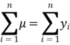
Since µ is a constant:

We have found the value of the constant:

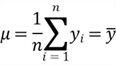
Through the least-squares method, we have found that the least-squares value for µ is the sample mean. Here is the equation for the line of the best fit:

where denotes the predicted value, i.e., an estimator of the mean value of the response variable.

With only one response variable, and no other information available, the sample mean is the best prediction for the mean number of orders that resulted from phone calls during a shift. The variability in the response variable can only be explained by the response variable itself [21]. We consider the horizontal line model to be the baseline model. When we introduce a predictor variable to the regression model, we expect the predictor variable can explain a portion of the variability. That is to say, the value of SSE from the simple linear regression model should be less than the SSE from the baseline model. Otherwise, the simple linear regression model is not significant; the predictor variable does not explain the variations in the number of orders.

In a horizontal line model, no other variable explains the variations in the observed response variable and, therefore, the SSE can represent the overall variations. To measure the total variability of a response variable for all kinds of linear regression modes, we use the sum of squares total, denoted SST [22]:

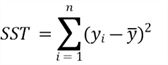
Plugging in the values in Table 2 into this equation, we obtain the SST of the response variable: SST = 423625.9. An essential purpose of data analysis is to explain the variability in a response variable. Without any other information about the response variable, we created a baseline model with unexplained total variability. For example, we cannot provide any information to explain why one shift generated 50 orders and another produced 487 orders. If we add other information, such as the number of phone calls received during a work shift, we can use this information to explain the variability and reduce SSE.

2.3.2 Simple Linear Regression

The horizontal line regression model does not have a meaningful explanation of the variations in the response variable. When we collect the number of phone calls received during a shift, shown in Table 1, we can use this number as a predictor variable to explain the observations that one work shift generated 50 orders, and another produced 487 orders. In order to use the least-squares method, we write the population regression model in a form of the sample regression model:

where the intercept and slope are unknown parameters. 

To estimate the parameters and , the sample regression model should make the value of SSE a minimum with respect to and :

We obtain the partial derivatives of SSE with respect to and :

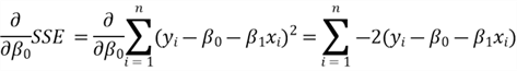
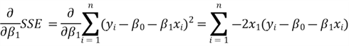
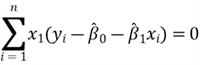
To find the minimum, we equate the two partial derivatives to zero. The least-squares estimators of and , denoted by and , respectively, must satisfy these two equations:

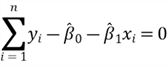
Since these two equations have two unknown variables, we can solve and [1]:

where is the sample correlation between X and Y, is the sample standard deviation of the X variable, and is the sample standard deviation of the Y variable. The symbols   and represent sample means of X and Y variables, respectively.

For the sake of simplicity, we also write the best-fitted line in this form:

Plugging data in Table 1 to equations solving for and , we obtain estimates for these two model parameters:

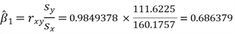
The model parameters we computed manually have the same values as those in the regression outputs shown in Figure 2. Using the sample regression model, we can obtain a point estimate of the mean of Y for a particular value of X.

We can now use the number of calls received during a shift to explain the variations in a response variable. As shown in Figure 6, our regression model does not capture all observed variations, but it does explain a portion of the variability. One shift generated 50 orders, and another produced 487 orders because these two shifts received different numbers of phone calls. Predicted values could be less than or higher than observed values. To measure how well the straight-line fits the sample data, we introduce a measure, sum of squares due to regression (or SSR). SSR is the sum of squared the differences between the predicted value and the response variable's mean:

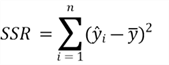
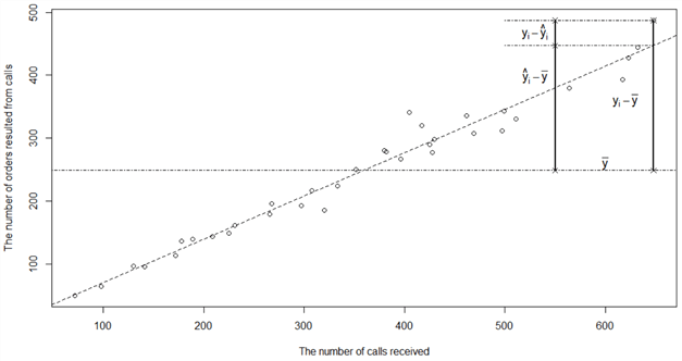
Figure 6 Measures the Explained Variability by the Line of Best Fit

Plugging data produced into this simple linear regression to the SSR and SSE equations, we obtain SST = 423625.9, SSR = 410960.5, and SSE = 12665.3. There is an apparent relation between SST, SSR, and SSE. After doing some algebra, we obtain this equation:

The total variability of the response variable consists of the explained and unexplained components. The higher value of SSR is, the more variations the regression model explained, and the better the regression line fits the data. When SST equals to SSR, that means the model explains all the observed variations. Otherwise, there is an unexplained component (or an error). Randomness, measurement error, or lack of other information could cause prediction errors.

2.3.3 Coefficient of Determination

The database table "FactCallCenter" has other columns, such as "TotalOperators," "AverageTimePerIssue," and "ServiceGrade." Because call center managers want to investigate connections between the number of orders and the number of calls, we hypothesized the simple regression model with the predictor variable "the number of calls." It is possible that the other columns also can be a predictor of Y. We usually consider a model that explains more variations in the response variable to be more useful.

To measure how much the predictor variable explains the total variability in a response variable, we use the ratio of SSR and SST. We call the rate as R-square, which has another name, "coefficient of determination."

We already know SST = 423625.9 and SSR = 410960.5; therefore, the R-square value is 0.97, which is the same as the value shown in Figure 2. We interpret the R-square as follows: when we predict the number of orders with the least-squares equation, the number of phone calls explains 97% of sample variations in the number of orders during a work shift. A considerable R-square value represents that the model fits well with the observed data because the regression model explains a large amount of variability in the response variable.

However, there is a problem with R-square. Even though we add unrelated predictor variables to the model, the R-square value stays the same or increases. Many researchers prefer the adjusted R-square, denoted by , which penalizes for having many parameters in the model. The concept of the adjusted R-square is not in the scope of this study. For completeness, this tip gives the equation to compute the adjusted R-square:

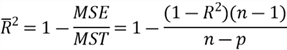
where MSE is Mean of Squares for Error, MST is Mean of Squares Total, n is the sample size, and p is the number of model parameters.

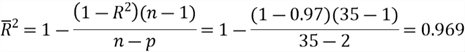
We use the following equation to compute the adjusted R-square for the simple linear regression model:

If we want to fit a straight line to the sample data, the least-squares approach has already helped us complete this task. Business users are interested in studying the population. When we want to draw inferences about the population from the sample data, we must invoke some distributional assumptions.

2.4 Perform Residual Analysis

We have hypothesized the simple linear regression model and used the least-squares method to find two estimators: and from the sample data. The true values of the intercept and the slope are unknown. We need to find out how well the two estimators approximate to the true parameters. The validity of many model inferences depends on the error component ε [8]. With the hypothesized model, we obtain the error component by rearranging the model equation:

It is worth noting that, in the simple linear regression analysis, given a value of X (i.e., ), the corresponding response variable and error term are random variables; furthermore, the random component ε determines the properties of . Since it is impractical to know the intercept and the slope , we cannot measure the error ε. However, we can use regression residuals, i.e., the differences between the observed Y values and predicted Y values, to estimate the random error ε [8]:

Residuals play an essential role in investigating model adequacy. We should always check the residuals of a regression model before we finally adopt the model for use. We use the following R function to glance at the regression residuals. The output from the R function is the same as the output in Figure 2.

> summary(residuals(model)) 
   Min. 1st Qu.  Median    Mean 3rd Qu.    Max. 
-36.712  -7.317  -1.574   0.000   8.171  60.946 
> 

2.4.1 Model Assumptions

In the simple linear regression model equation, the intercept and the slope are unknown constants and the random error component ε represents all unexplained variations in the response variable. We have the equation in Section 2.3.2 to obtain the estimator of the slope; we rewrite the equation in this form to discover the distribution of :

In preceding equation, is an independent and identically distributed () random variable, and the coefficient on each is a constant; therefore, is a linear combinations of random variables . We replace the with by using the fact that the response variable has a probability distribution at the point . The randomness of the error term reflects the randomness of the response variable ; therefore, we can discover the probability density function of the response variable from the error component . Consequently, we can relate the probability distribution of to the probability distribution of the error component. When we know the probability distribution of , we can obtain the probability distribution of . Thus, to make inferences about the parameters and , we must have some assumptions about the error component.

There are four standard assumptions about the error component of a linear regression model [2, 8]:

1. Unbiasedness: the mean value of the errors is zero in any thin vertical rectangle in the residual plot;
2. Homoscedasticity: the standard deviation of the errors is the same in any thin rectangle in the residual plot;
3. Independence: the errors associated with any two different observations are independent;
4. Normality: at any observation, the error component has a normal distribution;

Since any linear function of normal random variables is normally distributed [23, 24], the two model parameter estimators ( and ) have normal distributions under these four assumptions. These four assumptions are the basis for inferences in simple linear regression analysis; we can then develop hypothesis tests for examining the utility of the least-squares line and construct confidence intervals for predictions. For simplicity, I use equations in [25] to compute the standard error and t-statistic of the estimator :

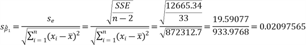
It is noteworthy that we use sample standard deviation to estimate the population standard deviation of the random error. The sample standard deviation is the square root of the sample variance. To obtain the sample variance, we divide the SSE by the number of degrees of freedom for this quantity. The number of degrees of freedom for error variance estimation is (n-p) when the regression analysis has n observations and p parameters. It is critical to verify these assumptions in practice since all inferences about these two parameters depend on these four assumptions. Because the true error component is unknown, we use the residuals to estimate the error component and, then, detect departures from these four assumptions.

2.4.2 Verify the Unbiasedness and Homoscedasticity Assumptions

Although we can perform formal statistical tests to check model assumptions, it is convenient to make visual inspections on residuals. Residual plots are useful to verify the unbiasedness and homoscedasticity assumptions. A residual plot, which is a scatter diagram, plots the residuals on the y-axis vs. the predicted values on the x-axis. We can also produce residual plots of the residuals vs. a single predictor variable. Professor Jost summarized six patterns of residual plots [2], shown in Figure 7. When a regression model satisfies the unbiased and the homoscedastic assumptions, its residual plot should have a random pattern, as illustrated in graph (a). Otherwise, the model may miss some predictors, or the linear model may not be the best technique for the data under analysis [26]. Several remedies are available for these kinds of assumption violations, such as X or Y data transformations.

Figure 7 Six Patterns of Residual Plots [2]

Assuming we have already constructed the simple linear model in R, we use the following script to produce a residual plot, as shown in Figure 8. We observe some outliers in the plot, but the residual plot pattern still approximates to be random.

# Get residuals and predicted values. 
residual.values <- residuals(model) 
predicted.values <- fitted(model) 

# Create residual plot.
plot(predicted.values, residual.values,           
     xlab ="Predicted numbers of orders during a shift", 
     ylab ="Residuals")
abline(h = 0, col ="red",  lty ="dotdash")

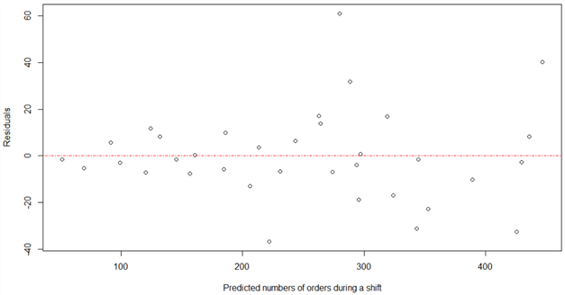
Figure 8 The Residual Plot of the Number of Orders Model

2.4.3 Verify the Independence Assumption

To demonstrate simple linear regression analysis, I purposely select one predictor, i.e., the number of calls received during a shift. As Professor Smith suggested [27], we should record any time or spatial variables when making observations since time or spatial correlations appear frequent. Regarding the call center data analysis, it makes sense to add two other predictor variables: date key, and work shift, to the regression model. Then, we can make the residual plots detect possible lack of independence. We can also use the Durbin-Watson test to test if there is a trend in the data based on previous instances.

The sample data set used for this exercise does not include a time or spatial variable. We can consider this data set to be a cross-sectional dataset that we collect data on entities only once. As Bansal pointed out [28], in cross-sectional datasets, we "assume" the model meets the independence assumption.

2.4.4 Check the Normality Assumption

We can use both formal statistical tests and graphical methods to check the normality assumption. When a model does not meet this assumption, formal statistical tests have low power [8]. Thus, we use graphical methods to check the normality assumption in this exercise.

The normal probability plot is a graphical technique for checking the assumption of normality. There are two versions of probability plots: Q-Q and P-P. In this study, we adopt the Q-Q plot that is a scatter diagram of the empirical quantiles of the residuals (y-axis) against the theoretical quantiles of a normal distribution (x-axis). If the Q-Q plot is close to a straight line, the probability distribution the residuals have is close to normal.

In practice, we need to determine the severity of the departures from normality. Professor Jost provided sketches of five normal plots and their interpretations [2], shown in Figure 9. We can compare the normal plot we obtained to these sketches then decide what remedial measure we should apply.

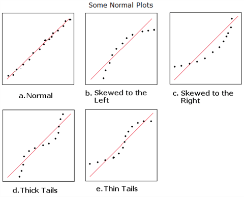
Figure 9 Sketches of Five Normal Plots and Interpretations [2]

We use the following script to produce a Q-Q plot, as shown in Figure 10. Based on Figure 9, the probability distribution of the residuals seems to have thick tails, which means residuals have more extreme values than expected if they have a normal distribution. When residuals do not have a normal distribution, we should apply some methods to rectify the model [29]. However, moderate departures from the normality assumption have minimal effect on the statistical tests and the confidence interval constructions. Therefore, the normality assumption is the least restrictive when we apply regression analysis in practice [8]. While systematic departures from normality are somewhat troubling, we still can move forward.

# Get residuals
resid <- resid(model) 

# Create Q-Q plot of residuals.
qqnorm(resid)
qqline(resid)

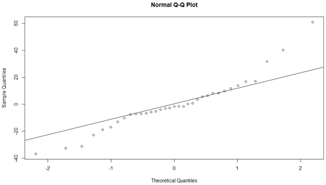
Figure 10 The Normal Q-Q Plot

2.5 Assess the Usefulness of the Model

When the response variable is completely unrelated to any identified predictor variable, we hypothesize a horizontal line regression model:

We have found the estimator of the average number of orders during all work shifts is about 249 in Section 2.3. During any work shift, the predicted mean of the number of orders that resulted from calls is 249. We are concerned that the number of calls received during a shift contributes information for predicting the response variable. In Section 2.1, we hypothesized a simple linear regression model:

In Section 2.3, we computed the true slope's estimator, , from the sample data.

2.5.1 Hypothesis Test for the Regression Slope

Based on the sample data, for every 100 phone calls during a shift, the average number of orders in the work shift increases by 69. The sample data reveal the influence of the number of calls on the number of orders. We want to ensure that we can observe the same impact in repeated sampling. We need to perform a test to verify whether the effect we have seen in one sample is significant or by chance. The null hypothesis is that the predictor variable X does not explain the variability of response variable Y (i.e., the horizontal line regression model). The alternative hypothesis is that X and Y have a linear relationship (i.e., the simple linear regression model). We choose a significance level of 0.05, which indicates a 5% risk of rejecting the null hypothesis when it is true.

We use the results from preceding calculations to perform the hypothesis testing and follow the five-step procedure introduced in [15]. Here is a list of inputs for the test:

• Sample size:
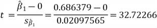
• The estimator of the slope:
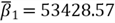
• The standard error of the slope:
• Null hypothesis value:
• The level of significance:

We follow the 5-step process to perform the two-tailed t-test:

Step 1: State the null and alternative hypotheses:

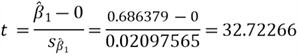
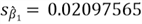
Step 2: Compute the test statistic:

Step 3: Compute (1-α) confidence interval for the test statistic t:

This hypothesis test is two-tailed, and therefore the 95% confidence interval is two-sided. Since the sample size is greater than 30, we use the standard normal distribution table to find the critical value. The critical value is 1.96 when α = 0.05. Thus, the 95% confidence interval for the test statistic is [-1.96, 1.96].

Step 4: State the technical conclusion:

Since the test statistic 32.7 lies outside of the interval [-1.96, 1.96], the test statistic is in the rejection area. The sample data provide sufficient evidence to reject the null hypothesis; therefore, we reject the null hypothesis at a significance level of 0.05. Consequently, we have significant evidence that is not 0.

Step 5: Compute p-value:

Use R function "pt" to compute the p-value.

> 2 * pt(-32.7, df = 35 - 2) 
[1] 1.007418e-26 
> 

Therefore, we have obtained the p-value:

When we repeat this experiment by using the same sampling process to obtain more samples, if the true slope is 0 (i.e., ), the chance of having a no more than 0.69 or no less than -0.69 is extremely small. There is very strong evidence against the null hypothesis in favor of the alternative hypothesis. The evidence extracted from sample data indicates that the number of calls during a shift contributes information for predicting the number of orders received from the work shift.

In practice, we may face a situation that we fail to reject the null hypothesis. This statistic conclusion does not lead us to accept the null hypothesis. This test result may imply a more complex relationship between Y and X.

2.5.2 Confidence Intervals for Linear Regression Slope

Even though we have found the estimator of the regression slope , there are some limitations. When we select other samples from the population, we have different values of the estimator. To make inferences about the slope , we should construct a confidence interval for the regression slope. We use the results from preceding calculations and follow a four-step procedure [14] to build a 95% confidence interval for the slope :

Step 1: Find the sample size, the estimator, and the standard error of the estimator.

• Sample size:
• Degrees of freedom:
• The estimator of the slope:
• The standard error of the slope:
• The level of significance:

Step 2: Compute the t-statistic.

Step 3: Obtain a 95% confidence interval for the t-statistic.

We use the R function qt() to obtain the 95% confidence interval for the t-statistic:

> qt(c(0.025, 0.975),df = 33) 
[1] -2.034515  2.034515 
> 

We write the interval in this format:

Plug the t-statistic into the inequality:

Step 4: Construct a 95% confidence interval for the for the slope by solving the inequality.

The interval [0.64, 0.73] is called a 95% confidence interval for the model slope . We are 95% confident that the interval [0.64, 0.73] contains the true . R provides the function "confint" to compute confidence intervals for one or more parameters in a fitted model. We use this function to verify our calculation and obtain the confidence interval for the intercept :

> confint(model, level = 0.95) 
                  2.5 %     97.5 % 
(Intercept) -14.6757899 18.8169778 
Calls         0.6437037  0.7290542 
> 

The R function outputs have the same interval as the result of our calculation. We also obtain the 95% confidence interval for the model Intercept , i.e., [-14.68, 18.82].

2.6 Apply the Model for Predictions

We have used residuals to check model adequacy. We now make predictions to ensure the results are acceptable. Bear in mind that, when we predict the response variable in terms of the predictor, the predictor's values should be within the original data set range. Let us review the least-squares model equation we found in Section 1:

For the sake of convenience, we use this general form:

The symbol stands for an estimator of the mean value of Y. We can use this equation to estimate the mean of Y, given a specific X value. Additionally, we can use this equation to forecast the best point estimate of Y value for a particular X value. For example, when the call center receives 200 phone calls in a shift, the predicted mean number of orders that resulted from phone calls is (2.07 + 200×0.69) ≈140. Meanwhile, the best point estimate of the number of customer orders is also 140. While both predictions have the same value (i.e.,140), they have different confidence intervals. The reason is that these two have distinct standard errors.

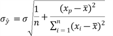
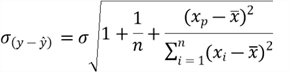
The standard error of the estimate for the mean of Y at the data point [8,25]:

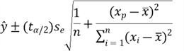
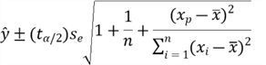
Therefore, we obtain a 100(1−α)% confidence interval for the mean value of Y for :

The standard error of the estimate for a single value of Y at the data point [8,25]:

Therefore, we obtain a 100(1−α)% confidence interval for predicting a single value Y for :

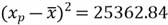
To find a 95% confidence interval for the mean number of orders when the call center receives 200 phone calls during a shift, we can plug the following values into the formula:

• 
• (based on DF = 33)
• 
• 
• 
• 

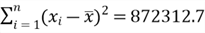
Then, we have:

This computation result means that we can be 95% certain that the interval [130.45, 149.55] contains the mean number of orders when the call center receives 200 phone calls during a shift. We use the following R function to verify our calculation:

> newdata <- data.frame(Calls = 200) 
> predict(model, newdata, interval = "confidence") 
       fit      lwr      upr 
1 139.3464 129.7766 148.9161 
> 

To find a 95% confidence interval for the number of orders when the call center receives 200 phone calls during a particular shift, we can plug the following values into the formula:

• 
• (based on DF = 33)
• 
• 
• 
• 

Then, we have

This computation result means we can be 95% certain that the interval [99.10, 180.90] contains the number of orders when the call center receives 200 phone calls during the particular shift. We use the following R function to verify our calculation:

> newdata = data.frame(Calls = 200) 
>  predict(model, newdata, interval = "prediction") 
       fit      lwr      upr 
1 139.3464 98.35593 180.3368 
>  

Because of the rounding error in our calculation, our results are slightly different from the results produced by the R script. We observe that two confidence intervals have different widths, and the confidence interval for the mean has a smaller width than the one for the single value. The following R program plots the shape of confidence intervals. The output of the program is shown in Figure 11. The confidence interval for the single value prediction is always larger than the mean value prediction interval. These two confidence intervals become narrowest at the mean value of X, increasing steadily as the distance from the mean increases. When we select an X value that lies outside the sample data range, the confidence interval is wide; therefore, the predicted values may not be meaningful.

# Makeup X values for predictions
sample.orders.min <- min(sample.orders$Calls) 
sample.orders.max <- max(sample.orders$Calls) 

# Include values fall outside of the sample data 
vector.new.values = seq(from = 0, to = sample.orders.max + 100, by = 40) 
data.frame.new.values = data.frame(Calls = vector.new.values) 
 
# Use the model to predict the number of orders for the data in data.frame.new.values 
data.frame.new.values$Orders <- predict(model, newdata = data.frame.new.values) 

# Obtain 95% confidence (Mean) limits 
data.frame.new.values$LoCI <- predict(model, newdata = data.frame.new.values,
                                      interval ="confidence")[, 2] 
data.frame.new.values$HiCI <- predict(model, newdata = data.frame.new.values,
                                      interval ="confidence")[, 3] 
 
# Obtain 95% prediction limits
data.frame.new.values$LoPI <- predict(model, newdata = data.frame.new.values,
                                      interval ="prediction")[, 2] 
data.frame.new.values$HiPI <- predict(model, newdata = data.frame.new.values,
                                      interval = "prediction")[, 3] 
 
# The attach function allows to access variables of a data.frame without calling the data.frame. 
attach(data.frame.new.values)

# Create the regression line.
plot(Calls, Orders, type ="l", col ="black", lwd = 2, 
        xlab ="Given values of X variable",
        ylab ="Computed Y values")

# Add 95% confidence (Mean) limits 
lines(Calls, LoCI, col ="blue", lwd = 2) 
lines(Calls, HiCI, col ="blue", lwd = 2) 

# Add 95% prediction limits
lines(Calls, LoPI, col ="red", lwd = 2) 
lines(Calls, HiPI, col ="red", lwd = 2) 

# Add sample data limits
lines(c(sample.orders.min, sample.orders.min), c(0, 600), lty = 4, col ="orange")
lines(c(sample.orders.max, sample.orders.max), c(0, 600), lty = 4, col ="orange")
legend("top", c("Regression Line","95% Confidence Limits",
                "95% Prediction Limits","The Range in Sample"),
                lty = c(1,1,1,4), lwd = c(2,2,2,1),
                col = c("black","blue","red",'orange'), y.intersp = 1.2) 

# Remove the attachment of the data.frame, 
detach(data.frame.new.values)

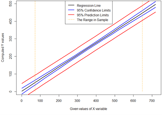
Figure 11 Confidence Internals Around the Regression Line

Examining those formulas of the confidence interval construction, we notice the component "1/n". This component reminds us that the width of the intervals becomes smaller as we increase the sample size. However, when the value of "1/n" approximates zero, this method cannot improve accuracy. To obtain more accurate predictions, we should build more sophisticated models, capturing the response variable's remaining variation.

Regression analysis can support a cause-and-effect relationship between the variables, but it cannot imply causality alone. Obtaining a useful model is not the primary objective of data analysis. Business users want the regression models to give them new insights into the business processes that generated the data.

We can now present this regression analysis to the managers and ask whether they can accept all results produced by the model. If they are satisfied with these results, they can adopt this model for use; otherwise, we go back to step one and repeat the six-step procedure.

Summary

To apply linear regression techniques and subsequently discover insights in the sample data for decision-making, IT professionals need to know the basics of statistics to precisely interpret regression models. This tip has presented the essential elements in a simple linear regression model analysis. This tip lays the groundwork for understanding and applying linear regression analysis in the business world.

We started this tutorial with an R program that found the least-squares equation from a sample. To explain that knowing programming skills alone is insufficient to perform practical data analysis, we referenced Drew Conway's Venn diagram of data science. We should stay away from the danger zone in the Venn diagram.

Next, we followed a six-step procedure to linearly relate the number of orders that a call center obtained in a work shift to the number of calls received. We explored an approach to hypothesize a form of the simple linear regression model and, then, introduced a rule of thumb to determine the sample size. This study used the least-squares method to determine the equation of a straight line that best fits the sample data. To emphasize the importance of residual analysis, we analyzed the probability distribution and standard error of . We further covered four standard model assumptions that are the basis for making model inferences.

Then, we performed a hypothesis test to assess the model's usefulness and constructed a 95% confidence interval of the slop . The assessment results indicate that the number of calls contributes information to predict the number of orders received from the work shift. We then used the model to make predictions. We also introduced two types of confidence intervals:  confidence (mean) intervals and prediction intervals.

In this tip, we used functions in the R programming language to verify our calculations. We additionally compared the model outputs from R to results from our computations. Although two approaches have obtained the same results, the manual process enhances our understanding of simple linear regression.

References

[1] Montgomery C. D., Peck A. E. & Vining G. G. (2012). "Introduction to Linear Regression Analysis (5^th Edition)," Hoboken, NJ: Wiley.

[2] Jost, S. (2017). CSC 423: Data Analysis and Regression. Retrieved from DePaul University: http://facweb.cs.depaul.edu/sjost/csc423/

[3] Porterfield, T. (2017). Excel 2016 Regression Analysis. Retrieved from YouTube: https://youtu.be/0lpfmFnlDHI/.

[4] Box, G. E. P. (1979). "Robustness in the Strategy of Scientific Model Building", Robustness in Statistics, pp. 201–236. New York, NY: Academic Press.

[5] Chauhan, S. N. (2019). A beginner's guide to Linear Regression in Python with Scikit-Learn. Retrieved from Towardsdatascience: https://towardsdatascience.com/a-beginners-guide-to-linear-regression-in-python-with-scikit-learn-83a8f7ae2b4f.

[6] Martin, R. Using Linear Regression for Predictive Modeling in R. Retrieved from Dataquest: https://www.dataquest.io/blog/statistical-learning-for-predictive-modeling-r/.

[7] Tracy, B. (2000). The 100 Absolutely Unbreakable: Laws of Business Success. San Francisco, CA: Berrett-Koehler

[8] William, M., & Sincich, T. (2012).  A Second Course in Statistics: Regression Analysis (7th Edition). Boston, MA: Prentice Hall.

[9] Zhou, N. (2018). Getting Started with Data Analysis on the Microsoft Platform - Examining Data. Retrieved from mssqltips: https://www.mssqltips.com/sqlservertip/5758/getting-started-with-data-analysis-on-the-microsoft-platform--examining-data/.

[10] Zhou, N. (2019). Numerically Describing Dispersion of a Data Set with SQL Server and R. Retrieved from mssqltips: https://www.mssqltips.com/sqlservertip/6058/numerically-describing-dispersion-of-a-data-set-with-sql-server-and-r/.

[11] Zhou, N. (2020). Basic Concepts of Probability Explained with Examples in SQL Server and R. Retrieved from mssqltips: https://www.mssqltips.com/sqlservertip/6278/basic-concepts-of-probability-explained-with-examples-in-sql-server-and-r/.

[12] Zhou, N. (2020). Selecting a Simple Random Sample from a SQL Server Database. Retrieved from mssqltips: https://www.mssqltips.com/sqlservertip/6347/selecting-a-simple-random-sample-from-a-sql-server-database/.

[13] Zhou, N. (2020). Using SQL Server RAND Function Deep Dive. Retrieved from mssqltips: https://www.mssqltips.com/sqlservertip/6301/using-sql-server-rand-function-deep-dive/.

[14] Zhou, N. (2020). Statistical Parameter Estimation Explained with Examples in SQL Server and R. Retrieved from mssqltips: https://www.mssqltips.com/sqlservertip/6301/using-sql-server-rand-function-deep-dive/.

[15] Zhou, N. (2020). Discovering Insights in SQL Server Data with Statistical Hypothesis Testing. Retrieved from mssqltips: https://www.mssqltips.com/sqlservertip/6477/discovering-insights-in-sql-server-data-with-statistical-hypothesis-testing/.

[16] Kess, B. (2017). AdventureWorks sample databases. Retrieved from GitHub: https://github.com/Microsoft/sql-server-samples/releases/tag/adventureworks/.

[17] Conway, D. (2015). The Data Science Venn Diagram. Retrieved from GitHub: http://drewconway.com/zia/2013/3/26/the-data-science-venn-diagram.

[18] Wasserman, L. (2004). All of Statistics: A Concise Course in Statistical Inference. New York, NY: Springer

[19] Frost, J. (2017). Choosing the Correct Type of Regression Analysis. Retrieved from Statistics by Jim: https://statisticsbyjim.com/regression/choosing-regression-analysis/.

[20] Hummelbrunner, S. A., Rak, L. J., Fortura, P., & Taylor, P. (2003). Contemporary Business Statistics with Canadian Applications (3rd Edition). Toronto, ON: Prentice Hall.

[21] Foltz, B. (2013). Statistics 101: Linear Regression, The Very Basics. Retrieved from Statistics 101: https://youtu.be/ZkjP5RJLQF4.

[22] Zeltzer, J. (2013). What is regression | SSE, SSR and SST | R-squared | Errors (ε vs. e). Retrieved from Z Statistics: http://www.zstatistics.com/videos#/regression.

[23] Hwang, J., & Blitzstein, K. J. (2015). Introduction to Probability. Boca Raton, FL: CRC Press.  

[24] Tsitsiklis, J. (2018). A Linear Function of a Normal Random Variable. Retrieved from MIT OpenCourseWare: https://ocw.mit.edu/resources/res-6-012-introduction-to-probability-spring-2018/part-i-the-fundamentals/a-linear-function-of-a-normal-random-variable/.

[25] Rawlings, O. J, Pantula, G. S, & Dickey, A. D. (1998). Applied Regression Analysis: A Research Tool (2^nd Edition). New York, NY: Springer.  

[26] Frost, J. (2017). Check Your Residual Plots to Ensure Trustworthy Regression Results! Retrieved from Statistics by Jim: https://statisticsbyjim.com/regression/check-residual-plots-regression-analysis/.

[27] Smith, K. M. (2012). COMMON MISTAKES IN USING STATISTICS: Spotting and Avoiding Them. Retrieved from utexas.edu: https://web.ma.utexas.edu/users/mks/statmistakes/modelcheckingplots.html/.

[28] Bansal, G. (2011). What are the four assumptions of linear regression? Retrieved from UW-Green Bay: https://blog.uwgb.edu/bansalg/statistics-data-analytics/linear-regression/what-are-the-four-assumptions-of-linear-regression/.

[29] Barker, L. E., & Shaw, K. M. (2015). Best (but oft-forgotten) practices: checking assumptions concerning regression residuals. The American journal of clinical nutrition, 102(3), 533–539. https://doi.org/10.3945/ajcn.115.113498.

[30] Kabacoff, R. (2015). R in Action, Second Edition: Data analysis and graphics with R. Shelter Island, NY: Manning Publications.

Next Steps

• The regression analysis involves techniques to establish relationships between a response variable and a group of predictor variables.  I purposely spent Section 1 on showing a way to find the linear regression equation. Some people may think that Section 1 completed a task of simple linear regression analysis. However, as Kabacoff mentioned [30], practical regression analysis is an interactive, holistic process with many steps, and it involves more than a little skill. Although I have discussed many elements in Section 2, this tip only serves as a starting point in linear regression analysis. With an adequate mathematical model, we can predict a response variable in terms of the predictor variables. In practice, the model is unknown; we must study the sample data and then make inferences about the population. Therefore, to build a useful model, we must know techniques for identifying potential problems with candidate models and making improvements. I referenced the danger zone illustrated in Drew Conway's Venn diagram of data science. To avoid the danger zone, we must learn the math and statistics behind the regression analysis. I have not provided all the mathematical derivations of formulas or equations used in this tip. Book [25] offers many mathematical derivations.
• Check out these related tips:
  • Getting Started with Data Analysis and Visualization with SQL Server and R
  • Getting Started with Data Analysis on the Microsoft Platform - Examining Data
  • Numerically Describing Dispersion of a Data Set with SQL Server and R
  • SQL Server 2017 Machine Learning Services Visualization and Data Analysis
  • Basic Concepts of Probability Explained with Examples in SQL Server and R
  • Selecting a Simple Random Sample from a SQL Server Database
  • Statistical Parameter Estimation Examples in SQL Server and R
  • Using SQL Server RAND Function Deep Dive
  • Discovering Insights in SQL Server Data with Statistical Hypothesis Testing
  • SQL Server 2016 R Services: Executing R code in Revolution R Enterprise

About the author

Nai Biao Zhou is a Senior Software Developer with 20+ years of experience in software development, specializing in Data Warehousing, Business Intelligence, Data Mining and solution architecture design.

This author pledges the content of this article is based on professional experience and not AI generated.

View all my tips