Problem
This tip provides an overview of why Neural Networks are not enough and why Recurrent Neural Networks (RNNs) are essential when dealing with sequential data, such as time series and natural language processing. However, beginners often struggle with how information flows through the network, especially with concepts like hidden states and vanishing gradients. This tip aims to provide a simplified introduction to RNNs, focusing on their structure and how they handle sequences.
Solution
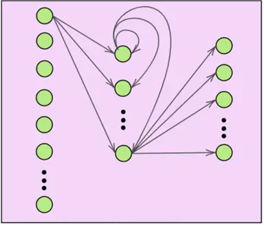
When data comes in the form of a sequence–word by word or image by image–we require a model architecture that can remember what happened a moment ago to make sense of what’s happening now. This is where a recurrent neural network (RNN) comes into play. In simple words, this new type of model provides our simple “vanilla” neural network with a memory mechanism, enabling it to read, listen, and predict with context rather than in isolation. In more formal words, RNNs are designed to process sequential input data by passing information from one step of the sequence to the next through hidden states, allowing the model to capture temporal dependencies and patterns that standard feed forward networks cannot. A general RNN is illustrated below, where the hidden states of the model can be observed as the ‘self-looping’ arrows in the nodes of the hidden layer of the network.
Shortcomings of Neural Networks
Rather than jumping right into what exactly RNNs are and how they work, we will instead be motivating their existence by highlighting why neural networks are inadequate for certain tasks. As highlighted before, our traditional neural networks treat every input in a ‘self-contained’ and independent manner. This means that they excel at recognizing patterns when the input size is fixed, e.g., a tabular dataset, because all relevant information is present simultaneously. However, when the data arrives piece by piece, its performance falls short. A stock price chart or a spoken sentence carry meaning in the order of its elements. If we are insensitive to this order of data, we will probably lose the very important insights we were hoping to learn in the first place.
Example
For a more concrete example, consider a language modelling task, where we aim to predict the next word considering the previous sequence of words. So, if our input data is “I woke up in the,” a good model should predict the next word as “morning.” In this example, we can see that the order of words is crucial to understanding the context and predicting what comes next. Each word contributes meaning not just on its own, but through its position and relationship to the words before it. Models like neural networks, however, fail to take word order into account and would treat “I woke up in the” the same as “in the I woke up” or “up the woke in I,” despite their vastly different meanings (or lack thereof).
Even if we force the input into the model, the network has no built-in notion of time. It processes every element independently, so it can’t naturally capture relationships with the elements of the input. For a neural network, the sentence “The dog chased the cat” is essentially the same as “The cat chased the dog,” even though these sentences convey entirely different scenes to us. In this regard, neural networks are often referred to as ‘stateless.’
Limitations of Neural Networks
Such limitations of neural networks primarily stem from the fact that they are fixed-input and fixed-output models. Recall that for a certain task, the number of input nodes (dataset features) and the number of output nodes (output classes in a dataset) are fixed at the time of model instantiation, training, and deployment. This, however, is a problem when it comes to sequence-based data, like sentences, audio clips, or time series, where inputs and outputs naturally vary in size. A very relevant example that demonstrates this is ChatGPT. We can prompt this language model with however many different sentences and words–it is not limited to, let’s say 10 words each time it is prompted. Similarly, the output that ChatGPT gives us also varies in the number of sentences and words each time. Likewise, if we wanted a neural network to translate a sentence from English to German, we’d struggle to fit both the variable-length input sentence and the variable-length translation into a fixed-size framework. This is because translation is inherently a variable sequence task, as one word in a language may be equivalent to a phrase of many words in another language.
This is why sequential models like RNNs are needed: they process ordered data one at a time, updating an internal memory at each step, which helps preserve the structure and context of the sequence. This allows them to make predictions that reflect the actual flow of sequential data.
Understanding How RNNs Work
Now that we have a background on why a model like RNN is needed, it is time to understand how exactly it works. For simplicity, we will build our explanation from a simple, 2-layer neural network, as depicted below.
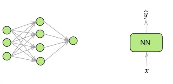
As you already know, this neural network has 1 hidden layer with 4 nodes, followed by an output layer with a single node. For simplicity, rather than redrawing the entire network again and again, we will be using the simpler block diagram as shown above.
Explanation
For our example, you can think that this neural network is designed to classify movie reviews into positive and negative sentiment. Normally, neural networks are capable of text sentiment classification, however, the words and sentences cannot be directly passed into the model. Feature extraction techniques like bag of words or a simple count of negative and positive words are used to transform textual data into order-invariant features that a neural network can ingest. As we just discussed previously, this will again reduce the performance of the network, as text is sequential data where the ordering of words carries a lot of meaning. So, for now, this neural network is designed to accept a single word as an input.
You may notice that the input layer of the network comprises 3 nodes. Although this topic requires another advanced discussion, you can think of a unique 3-dimensional vector representing each word. These are known as ‘word embeddings,’ and they are essentially mathematical, numerical representations of words, as machine learning models work with numbers, not text.
Expanding Scope
Moving on. So far, we have designed a neural network that can ingest and process a word. However, this is nowhere near achieving our task of movie review sentiment classification, as our network is only able to process one word, without any contextual and temporal information about the entire sentence in a particular movie review.
How do we transform this vanilla neural network into an Recurrent Neural Network that can accomplish just that? At the heart of an RNN is the concept of recurrence. The idea is that the output at each time step is influenced not just by the current input, but also by the past. Unlike traditional neural networks, which process input all at once, RNNs work step by step through a sequence, maintaining an internal hidden state that acts as memory. This hidden state is updated at each step, allowing the network to build up context over time and maintain a short-term memory of the data sequence.
Convert Neural Network to RNN
To convert our neural network above into an RNN, we simply need to introduce a hidden state, which is essentially just the output of the hidden layer of the neural network, fed into the same hidden layer in the next time step. This model is illustrated below:
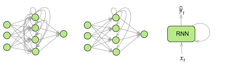
This may seem like a lot to unpack! Let’s dissect this diagram step by step. The first diagram is a complete depiction of what the nodes and layers in an RNN look like. It is updated from our previous vanilla network to include outputs of nodes in the hidden layer going to themselves and all other nodes in the hidden layer as an additional input in the next time step. As the first diagram is rather convoluted, this is better illustrated by the second diagram, where only one node’s recurrence is illustrated. Lastly, for simplicity, we will be going forward with the block diagram as shown in the third diagram.
Understanding the Processing
Now, we finally have a network that can decide the sentiment of movie reviews while maintaining memory about the context and order of the words in a given review. To understand an overview of how an RNN processes the input to output, let’s consider an example movie review: “Terrible movie until plot twist.” Now, a vanilla neural network is likely to classify this review as negative, even though it carries positive connotations. We know that the movie was terrible, but perhaps the plot twist changed that, and the movie turned out to be good. Let’s see how an Recurrent Neural Network may also reach the same conclusion. The diagram below illustrates how this review is processed by the model:
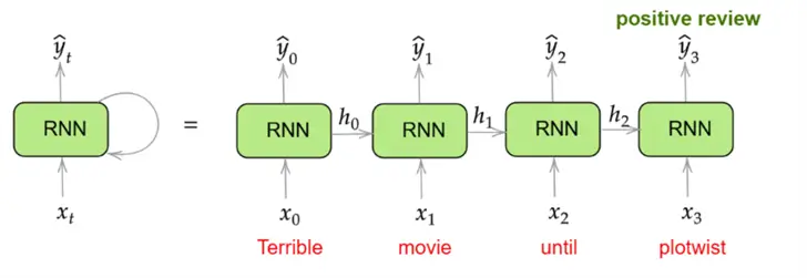
In this diagram, we have essentially unrolled the RNN to depict its working for all timesteps simultaneously. Note that the different RNN blocks above do not represent separate RNN models. It is the same model being shown for each timestep, with the same weights and activation functions.
The Steps
At the 0th time step, the model takes the input “Terrible” in the form of its 3-dimensional embedding. Since this is the first input word, the hidden state at this point is initialized to 0. This input is processed by multiplying it with the weights of the network in the hidden layer to produce the hidden state  . The model then moves to the next time step where the word “movie” and the hidden state from the previous time step
  are taken as input to produce
  . The model similarly processes the word “until” and
  as input, to produce
  for the final time step. Here, the final word “plotwist” and previous hidden state
  are processed to produce
  , which is then used to derive the final output
  .
.
The example in the image demonstrates how an Recurrent Neural Network processes a sentence word by word, updating its internal state at each step to capture the evolving context. Starting with “Terrible” and “movie,” the network initially leans toward a negative sentiment. However, when it encounters the word “until,” it begins to anticipate a shift in meaning and thus updates its internal state to reflect a more positive sentiment. This accumulated understanding allows the model to correctly interpret the overall sentiment of the review as positive, something a neural network, which treats inputs as fixed and context-free, would struggle to capture. The RNN’s ability to carry forward information through hidden states is what enables it to grasp complex patterns in sequences like natural language.
Sequences
Lastly, if you are wondering about the relevance of  ,
,  , and
, and  from the above example, here’s a simple answer: In many sequence tasks like the above sentiment classification example, we only care about the final output (e.g., predicting the overall sentiment at the end of a sentence). In such cases, the intermediate outputs like
  ,
,  , and
, and  are simply discarded because they reflect partial understanding based on incomplete context. However, there are other tasks (referred to as sequence-to-sequence tasks) where these intermediate outputs are of prime importance, such as translation, parts of speech tagging, etc.
The RNN Algorithm
Since we have already given a high-level, intuitive overview of RNNs, it is time to translate that into mathematics using our previous text sentiment example.
Forward Pass
In this step, the input sequence is processed to produce an output. For all time steps  ranging from
  , the following steps are repeated:
- At the t timestep, the
 hidden state
  is produced by the following equations:

Both the inputs  and
and  have their own distinct weight matrices, which are used to compute
  . Just like in neural networks, this linear combination of weighted input is passed through an activation function, which is hyperbolic tan in our example.
- The hidden state at time step
 ,
,  is then used to produce an output, through the following equation:

- At each time step
 , the output
  is evaluated using a reasonable loss function to produce the loss
  .
.
As discussed before, depending on the nature of the sequence task, either all the intermediate outputs ranging from  ,
,  ,
,  , …,
, …,  are concatenated to form the final output, or only the final output
  is saved. Similarly, the losses for each time step is also combined (e.g., mean can be taken) to form a single uniform measure.
Backward Pass
The algorithm to find an optimal set of weights for Recurrent Neural Network through gradient descent is called backpropagation through time. It is very complicated to be understood intuitively, given the dependency of output across all elements of sequence, and therefore is beyond the scope of this tip. However, the basic intuition remains the same: through calculus and optimization techniques, we hope to find a set of parameters that minimize the global loss of our model. The complication in this algorithm is primarily in finding the derivatives of loss function with respect to the parameters. Fortunately, we have frameworks like PyTorch, where we do not have to tussle with this concept in detail.
Implementing a Basic RNN in Python
Now that we have a complete theoretical understanding of RNNs, it is time to test that knowledge in a practical setting. Therefore, we will work with the Large Movie Review Dataset created by Maas et al. for a movie review sentiment classification using a vanilla Recurrent Neural Network. We will accomplish this task using the PyTorch framework for concise, readable, and reliable code.
Thus, to get started, we will be importing the required libraries.
#MSSQLTips.com (Python)
import pandas as pd
import re
from collections import Counter

import nltk
from nltk.corpus import stopwords
nltk.download('punkt')
nltk.download('punkt_tab')
nltk.download('stopwords')

import torch
from torch import nn
from torch.utils.data import Dataset, DataLoader
from torch.nn.utils.rnn import pad_sequence, pack_padded_sequence, pad_packed_sequence

from sklearn.model_selection import train_test_split
from tqdm import tqdm
We also need to initialize some hyperparameters for our model later on.
#MSSQLTips.com (Python)
BATCH_SIZE      = 64
EMB_DIM         = 128
HIDDEN_SIZE     = 128
N_EPOCHS        = 15
LR              = 1e-3
MIN_FREQ        = 2
MAX_VOCAB       = 30_000
DEVICE          = 'cuda' if torch.cuda.is_available() else 'cpu'
We can now import our dataset and inspect its dimensions.
#MSSQLTips.com (Python)
data = pd.read_csv('/content/IMDB Dataset.csv')
print("Shape: ", data.shape)
data.head()
As we can see, this dataset comprises 50,000 total observations with a column for the review itself, and a corresponding sentiment column.
Check for Missing Values
To ensure that there are no missing values in the dataset, we run the following command:
#MSSQLTips.com (Python)
data.isna().sum()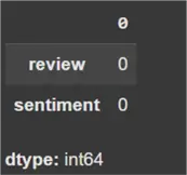
Since there are zero missing values in the dataset, we can move on to the next step.
Inspect Dataset for Uniform Class Distribution
We now need to inspect whether the dataset has uniform class distribution. In the latter’s case, the model performance might decrease as one class is overrepresented, which demands the need for additional sampling techniques to fix the problem. Fortunately, as we can see below, there is no need to undertake this step as the dataset is evenly representative of both sentiment classes.
#MSSQLTips.com (Python)
data['sentiment'].value_counts()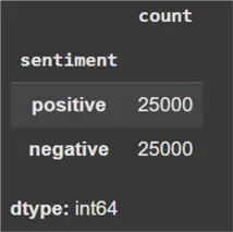
We can also observe that the sentiment is currently being stored in the form of textual labels. Let’s convert them to numerical labels for ease of use, where ‘1’ indicates positive and ‘0’ is negative.
#MSSQLTips.com (Python)
data['sentiment'] = data['sentiment'].apply(lambda x: 1 if x == 'positive' else 0)
Cleaning Data
As usual with textual data, it needs to be cleaned before it’s ready for classification. Therefore, we define a cleaning pipeline, which removes HTML tags, hyperlinks, extra white spaces, special characters, and stop words from the reviews before tokenizing it. In particular, we are using a word tokenizer that splits each review into individual words, as evident by the name.
#MSSQLTips.com (Python)
stop_words = set(stopwords.words("english"))

def clean(text):
    text = text.lower()

    text = [word for word in text.split() if word not in stop_words]  # remove stopwords
    text = " ".join(text)

    text = re.sub(r"<.*?>", "", text)  # remove HTML tags like <br>, </div>, etc.
    text = re.sub(r"https?://\S+|www\.\S+", "", text)  # remove hyperlinks
    text = re.sub(r"[^a-z\s]", "", text)  # remove digits and special characters

    text = " ".join(text)

    return text

#Tokenization pipeline
def tokenize(text: str):
    text = clean(text)
    return nltk.word_tokenize(text)
#MSSQLTips.com (Python)
texts = data['review'].tolist()
labels = data['sentiment'].tolist()
tokens_list = [tokenize(t) for t in tqdm(texts, desc="Tokenising")]
Vocabulary Building Process
We now move on to the vocabulary-building process that assigns each unique word an integer index. To do this efficiently and meaningfully, we first count the frequency of all tokens and then retain only the most common ones that appear frequently enough. This filtering helps reduce noise from typos or very rare words and prevents the model from overfitting to outliers. We also set an upper limit on vocabulary size to keep the model lightweight and manageable.
Additionally, we introduce special tokens: <pad> for sequence padding, to make all input sequences the same length in a batch, and <unk> for unknown or rare words not seen during training. Each token in the vocabulary is mapped to a unique integer in a dictionary called ‘stoi’ (string-to-index), which converts the input text into numerical sequences.
This step is essential to construct the word embeddings, where each word is transformed into a learnable dense vector representation, suitable for input into the RNN, bridging the gap between raw textual data and the numerical data required by models.
#MSSQLTips.com (Python)
counter = Counter(t for tokens in tokens_list for t in tokens)
common = [w for w, c in counter.items() if c >= MIN_FREQ][:MAX_VOCAB-2]
stoi = {"<pad>": 0, "<unk>": 1, **{w: i+2 for i, w in enumerate(common)}}
itos = {i: w for w, i in stoi.items()}
VOCAB_SIZE = len(stoi)
We also define a dataset class for loading the dataset efficiently into the model in batches. The dataset is also split into 80-20 train-test split.
#MSSQLTips.com (Python)
class IMDBDataset(Dataset):
    def __init__(self, token_lists, labels):
        self.data = token_lists
        self.labels = labels
    def __len__(self): return len(self.data)
    def __getitem__(self, idx):
        tokens = self.data[idx]
        ids = [stoi.get(tok, stoi["<unk>"]) for tok in tokens]
        return torch.tensor(ids, dtype=torch.long), torch.tensor(self.labels[idx], dtype=torch.float32)

def collate(batch):
    seqs, labs = zip(*batch)
    lengths = torch.tensor([len(s) for s in seqs])
    seqs_padded = pad_sequence(seqs, batch_first=True, padding_value=stoi["<pad>"])
    return seqs_padded, lengths, torch.stack(labs)
#MSSQLTips.com (Python)
train_x, val_x, train_y, val_y = train_test_split(tokens_list, labels, test_size=0.2, random_state=42, stratify=labels)
train_ds, val_ds = IMDBDataset(train_x, train_y), IMDBDataset(val_x, val_y)
train_dl = DataLoader(train_ds, batch_size=BATCH_SIZE, shuffle=True, collate_fn=collate)
val_dl = DataLoader(val_ds, batch_size=BATCH_SIZE, shuffle=False, collate_fn=collate)We can now start by defining our model with an RNN layer and begin training it with AdamW optimizer, alongside a learning rate of 1e-3 and 15 epochs.
#MSSQLTips.com (Python)
class RNN(nn.Module):
    def __init__(self, vocab_size, emb_dim, hidden_size):
        super().__init__()
        self.embed = nn.Embedding(vocab_size, emb_dim, padding_idx=stoi["<pad>"])
        self.rnn   = nn.RNN(emb_dim, hidden_size, batch_first=True)
        self.fc    = nn.Linear(hidden_size, 1)
    def forward(self, x, lengths):
        em = self.embed(x)
        packed = pack_padded_sequence(em, lengths.cpu(), batch_first=True, enforce_sorted=False)
        _, hn = self.rnn(packed)
        out = self.fc(hn.squeeze(0))
        return out.squeeze(1)
#MSSQLTips.com (Python)
def accuracy(preds, y):
return (torch.sigmoid(preds).round() == y).float().mean().item()
def run_epoch(model, loader, optim=None):
is_train = optim is not None
total_loss = total_acc = n = 0
model.train(is_train)
for X, lens, y in loader:
X, lens, y = X.to(DEVICE), lens.to(DEVICE), y.to(DEVICE)
out = model(X, lens)
loss = nn.BCEWithLogitsLoss()(out, y)
if is_train:
optim.zero_grad()
loss.backward()
optim.step()
total_loss += loss.item() * len(y)
total_acc += accuracy(out, y) * len(y)
n += len(y)
return total_loss/n, total_acc/n #MSSQLTips.com (Python)
model = RNN(VOCAB_SIZE, EMB_DIM, HIDDEN_SIZE).to(DEVICE)
optimizer = torch.optim.AdamW(model.parameters(), lr=LR)
for epoch in range(1, N_EPOCHS+1):
train_loss, train_acc = run_epoch(model, train_dl, optimizer)
val_loss, val_acc = run_epoch(model, val_dl)
print(f"[{epoch}/{N_EPOCHS}] "
f"train loss {train_loss:.4f} acc {train_acc:.3f} │ "
f"val loss {val_loss:.4f} acc {val_acc:.3f}")
And we are done! Although an accuracy of 65% might not seem impressive at first, recall that this model is still likely performing miles better than a neural network. Also, remember that Recurrent Neural Network is still a simpler model in the family of sequence models, and better results can be achieved by using advanced models.
Conclusion
In this tip, we gave a detailed theoretical overview of RNNs and motivated their development by highlighting the shortcomings of neural networks. To make the readers more comfortable, we used a practical demonstration using PyTorch in Python to implement an Recurrent Neural Network for a movie review sentiment classification.
Next Steps
- The interested readers should play with the code above and try to improve the model’s performance beyond 65%. They can try changing the learning rate, the number of epochs, using pre-trained embeddings, and even revising the text cleaning strategy.
- For the mathematical geniuses, they can investigate the exact mechanism in the backward pass of RNNs and try implementing the algorithm from scratch.
- To checkout more AI related tips.

 is produced by the following equations:
 is evaluated using a reasonable loss function to produce the loss
  .
.
