Problem
While Recurrent Neural Networks (RNN) are powerful, they often struggle with long-term dependencies due to the vanishing gradient problem. Long Short-Term Memory Networks (LSTMs) address this issue by introducing memory cells and gates. For beginners, understanding LSTM components, such as the input, output, and forget gates, can be challenging. This tip breaks down LSTMs in an intuitive way, highlighting their importance and practical applications.
Solution
While RNNs are designed to allow models to process sequences by retaining information from previous time steps, they often struggle with longer sequences of input data, and the model performance is thus subpar. As observed in our last tip, despite the impressive architectural advances of RNNs, our model was only able to achieve a mediocre accuracy of 65% in a movie review sentiment classification task. Thus, this is where Long Short-Term Memory networks (LSTM) come into play.
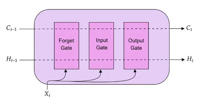
In simple words, LSTMs are a smarter version of RNNs that can selectively remember and forget information over long sequences. They come with a built-in “memory cell” and special structures called gates that control the flow of information—what to keep, what to update, and what to discard—allowing them to understand context over much longer spans than traditional RNNs. A high-level overview of a basic LSTM unit is illustrated below.
Shortcomings of Recurrent Neural Networks
Once again, rather than diving right into the equations, algorithmic steps, and the mathematical workings of LSTMs, let’s start by motivating this model’s existence instead. Similar to how the limitations of neural networks led to the need and development of RNNs, the shortcomings of RNNs led to architectural innovations, which ultimately yielded LSTMs in the machine learning ecosystem.
What are limitations
So, what are the limitations of RNNs in processing sequential data? Many of these limitations naturally stem from how the architecture of RNN is designed, particularly its backpropagation algorithm. Recall that the Backpropagation Through Time (BPTT) algorithm is the adaptation of the standard backpropagation algorithm used to train neural networks, but applied to RNNs instead, where the network unfolds over time. An interesting aspect of this algorithm is that each gradient at time step  does not only involve the derivatives of time step , but all the previous time steps as well, ranging from
  , with results concatenated through long chains of multiplications. Thus, as gradients are multiplied through multiple layers and multiple time steps simultaneously, the problem of unstable gradients naturally arises.
Walk Through Scenarios
To illustrate this, let’s walk through two different scenarios. Consider the following chain of multiplication:  . The answer is
  . Now, imagine that each individual digit above is a gradient being multiplied in the BPTT algorithm. In this example, you may have noticed that all of the gradients are between the range 0 and 1, and when such numbers less than 1 are multiplied together over long chains, we end up with a very ridiculously small number in the end! The longer the chains, the faster the resulting number will tend to zero. Although our example only involves five multiplications, we typically work with much longer sequences involving thousands or even millions of such multiplications!
This presents us with a serious problem, as modern computers only have finite precision. In other words, they have a physical limit to the smallest real number they can store and process. If during the BPTT algorithm, gradients become closer and closer to zero, and fall below this limit, numeric underflow can occur, and the gradients’ values are rounded to zero. This is termed the vanishing gradient problem. As the gradients become zero, the model stops learning any further, and the training stagnates. For this reason, an RNN is sometimes very difficult to train to achieve optimal results. This problem is further exacerbated if sigmoid activation function is used in the hidden layers of RNN, as the derivative of sigmoid function always lies between 0 and 1.
Exploding Gradient Problem
Similarly, an RNN can also run into the exact opposite issue, called the exploding gradient problem. Similarly, consider a very long chain of multiplication composed of large numbers like  and so on. Obviously, the end result of this multiplication would be humongous, and the number would tend closer and closer to infinity. Or the longer the input sequence is, the larger the gradients become. Like before, if this number exceeds the limit of what the computer can physically store in its memory, we run into a numeric overflow problem where the number is too large to be stored, and thus is truncated, reflecting another inaccurate number entirely. This results in unstable training and wildly fluctuating weight updates, preventing the model from converging. Although a technique known as gradient clipping can mitigate this problem somewhat, it does not solve the underlying structural issue of RNNs, due to which unstable gradients arise.
Additional Issues
Furthermore, a big limitation of RNNs is that they are simply not very good at capturing long-range dependencies in an input sequence. Consider the following movie review: “The movie’s beginning was slow and filled with clichés; however, it ultimately delivered a powerful story with a satisfying conclusion.” Although this review has mixed sentiment, starting off with a negative tone and ending with a positive, an RNN will fail to capture this multifaceted sentiment. This is because, although an RNN will process the entire input sequence, the information encoded in hidden states tends to be fairly local, reflecting the later parts of the sequence more than the earlier parts. As such, the information in the hidden states reflecting the starting words begins to get washed out and dominated by the recent words in the sequence, and thus the model begins to ‘forget’ the initial state of the sequence, preventing it from capturing long-range dependencies.
To address these issues pertaining to unstable gradients and inability of RNNs to capture the underlying relationship between sequences, more complex network architectures, like LSTMs, have been designed to explicitly manage the task of maintaining relevant memory over time. They do this by allowing the network to learn to forget irrelevant information while retaining relevant information that may be required for the model’s decision-making in the subsequent time steps.
Algorithm and Theory of LSTMs
Now that we have an understanding of why LSTMs are needed, let’s probe into how they actually work. In more formal words, LSTMs are a type of RNN specifically designed to overcome the limitations of standard RNNs by incorporating memory cells and gating mechanisms. The function of gates is essentially to control the flow of information through the network by determining what information to store, forget, and output, respectively.
At its core, an LSTM cell maintains two types of memory:
- Cell state
 : Acts like a conveyor belt, carrying long-term memory through the sequence with minimal modifications.
 - Hidden state : Reflects the short-term memory of the cell.
 : Acts like a conveyor belt, carrying long-term memory through the sequence with minimal modifications.
 : Reflects the short-term memory of the cell.
Below is a detailed illustration of an LSTM unit, showing how an input sequence at a time, step , is processed as it passes through different gates.
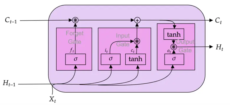
At each time (step ), the LSTM takes in the input vector  (e.g., a contextualized embedding for a word from a sentence), previous hidden state
  (short term memory), and previous cell state
  (long term memory). After these inputs are processed as they flow through the three gates (forget gate, input gate, and the output gate), the LSTM outputs the updated hidden state
  and cell state
  .
.
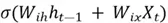
Let’s step into each gate one by one to inspect the LSTM under the hood. Before we begin, it is important to acknowledge that each gate has its own unique sets of weight matrices that are not shared with other gates. However, across different time steps, these matrices remain the same just like in RNNs.
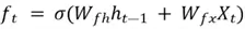
Forget Gate
The primary function of the forget gate is to manage which information to forget from the cell state. The outcome of this decision is a selector vector  computed as below:
Where  and
and  are the weight matrices in the forget gate.
Since the weighted sum of the previous hidden state and the input vector is passed through the sigmoid activation function, our output will comprise a vector, whose elements are between 0 and 1. For this reason, is called a selector vector, as the value of its elements will directly dictate what percentage of information to forget from the previous cell state. For instance, if  primarily has values close to 1, most of the content of will be retained. On the other hand, if the selector vector has smaller values close to 0, most of the information will be forgotten.
This latter step is enforced by multiplying the selector vector with the cell state vector to produce a partially updated cell state vector  :
:
The  symbol denotes Hadamard product, which is simply the element-wise product of two matrices of the same dimensions. An example is outlined below:
Suppose that  and
and =
=
Then 
To summarize, this gate allows the LSTM to forget irrelevant past information, such as old context that is no longer relevant to future decisions. By selectively forgetting old, irrelevant context, LSTMs can shift focus to what is most important—something critical in language, where meanings often change based on what comes later.
Input Gate
After forgetting the irrelevant information from the cell state, the LSTM also has to update it with additional information from the current time step. This action is completed in three steps in the input gate.
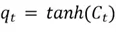
Step 1. First, a candidate memory vector  is generated by passing a weighted sum of the previous hidden state and input vector to the hyperbolic tan activation function:
=
Where  and
and  are the weight matrices for candidate memory generation in the input gate.
Since the hyperbolic tan activation function is used, the value of the candidate memory vector will range from -1 to 1.
Step 2. Then, a selector vector  is produced to control which part of the new candidate memory should be added to produce the updated cell state. As discussed before, since a selector vector by design is supposed to monitor proportions of the vector it is multiplied with, it is natural to use the sigmoid activation function as it ranges between 0 and 1. Thus, is constructed as follows:
= 
Where  and
and  are the weight matrices for the selector vector in the input gate.
Now, this selector vector can be used to determine what chunk of the candidate memory is relevant:

Where  is a vector representing the updated candidate memory.
Step 3. To produce the updated cell state , we simply have to add this updated candidate memory and the partially updated cell state vector that was produced by the forget gate:

In short, these steps allow the LSTM to add new relevant information to the long-term memory.
This linear flow through the cell state is what allows gradients to be preserved, reducing the problem of unstable gradients.
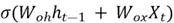
Output Gate
Now that the cell state for the current time step is updated, the LSTM has to update the hidden state as well. Similar to the input gate, the updated hidden state is also produced from a multiplication between the candidate vector and a selector vector.
The candidate hidden state vector  is computed as follows:
Where  is the updated cell state from the input gate.
Like earlier, the selector vector is also generated based on values of and  :
:
 =
= 
Finally, the updated hidden state can be computed by multiplying the selector and candidate vector:
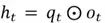
To wrap up, the output gate generates the updated hidden state , which can be passed to the next time step or used to make predictions by the LSTM network.
One reason for the failure of RNNs to maintain a long-term context and carry forward critical information was due to the fact that these hidden states were not only providing information to generate output at the current time step but also updating and carrying information for future timesteps simultaneously. On the other hand, as we have just discussed, LSTM can directly manage the relevant context over time by splitting the task of maintaining information for current decisions through the hidden state vector , and information that is to be passed to future time steps in the form of long-term memory .
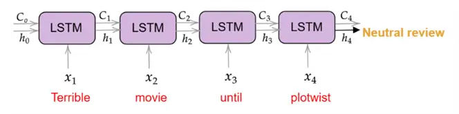
LSTM Processing
Zooming out of the individual LSTM unit, it is time to inspect how the model processes an entire input sequence. Suppose we are working with a movie review “Terrible movie until plotwist.” As illustrated below, at each time step, the LSTM ingests a word and processes it using the previous hidden and cell state, producing the updated memory states as output, which are then used as an input in the next time step. At the last time step, the model employs the final hidden state  to make a decision regarding the review’s sentiment, which turns out to be neutral in this case.
Lastly, again due to rising complexity, we will not be covering the backpropagation algorithm for LSTMs. However, it is important to keep in mind that the network is trained to learn what to remember and forget through the BPTT algorithm.
Implementing a Simple LSTM Model in Python
Now that we have a basic level of familiarity with LSTMs, it is time for a practical demonstration with Python. In this section, we will once again be working with the Large Movie Review Dataset created by Maas et al. for a movie review sentiment classification using a Bidirectional LSTM (BiLSTM) model in PyTorch for concise, readable, and reliable code.
A BiLSTM model simply comprises two LSTM layers that process the text in both forward and backward directions, allowing the model to grasp the underlying semantics much better.
Import Libraries
Thus, let’s start by importing relevant libraries and modules.
#MSSQLTips.com (Python)
#Required libraries
import pandas as pd
import re
from collections import Counter

import nltk
from nltk.corpus import stopwords
nltk.download('punkt')
nltk.download('punkt_tab')
nltk.download('stopwords')

import torch
from torch import nn
from torch.utils.data import Dataset, DataLoader
from torch.nn.utils.rnn import pad_sequence, pack_padded_sequence, pad_packed_sequence

from sklearn.model_selection import train_test_split
from tqdm import tqdm
We also need to initialize some hyperparameters for our model later on.
#MSSQLTips.com (Python)
#Hyperparameters
BATCH_SIZE      = 64
EMB_DIM         = 128
HIDDEN_SIZE     = 128
N_EPOCHS        = 15
LR              = 1e-3
MIN_FREQ        = 2
MAX_VOCAB       = 30_000
DEVICE          = 'cuda' if torch.cuda.is_available() else 'cpu'
Load and Inspect Dataset
Now, we can load and inspect our dataset. It contains two columns: one for the review itself and the other for the corresponding sentiment.
#MSSQLTips.com (Python)
data = pd.read_csv('/content/IMDB Dataset.csv')
print("Shape: ", data.shape)
data.head()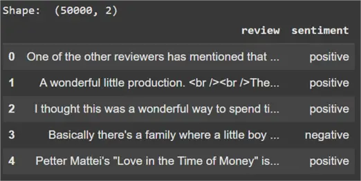
This dataset consists of 50,000 total observations. Before moving forward, it is also important to check whether we are working with a binary classification problem or not.
#MSSQLTips.com (Python)
#Label distribution
data['sentiment'].value_counts()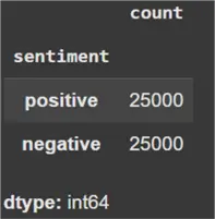
Since there are only two labels in the sentiment column, it confirms that we are working with a binary classification setup.
Clean Dataset
Before we can move towards model defining and building, it is imperative that we clean our dataset first and foremost. To get started, we check for any missing values in the dataset.
#MSSQLTips.com (Python)
#Checking for null values
data.isna().sum()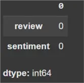
As we can see above, there are zero null values in the dataset.
We can also observe that the sentiment is currently being stored in the form of textual labels. Let’s convert them to numerical labels for ease of use, where ‘1’ indicates positive and ‘0’ is negative.
#MSSQLTips.com (Python)
#Converting the labels from string to integer
data['sentiment'] = data['sentiment'].apply(lambda x: 1 if x == 'positive' else 0)
Now we can clean our text data. For this step, we define a cleaning pipeline that removes HTML tags, hyperlinks, extra white spaces, special characters, and stop words from the reviews before tokenizing it. In particular, we are using a word tokenizer that splits each review into individual words, as evident by the name.
#MSSQLTips.com (Python)
#Text preprocessing
stop_words = set(stopwords.words("english"))

def clean(text):

    text = text.lower()
    text = [word for word in text.split() if word not in stop_words]  # remove stopwords
    text = " ".join(text)

    text = re.sub(r"<.*?>", "", text)  # remove HTML tags like <br>, </div>, etc.
    text = re.sub(r"https?://\S+|www\.\S+", "", text)  # remove hyperlinks
    text = re.sub(r"[^a-z\s]", "", text)  # remove digits and special characters

    text = " ".join(text)

    return text

#Tokenization pipeline
def tokenize(text: str):
    text = clean(text)
    return nltk.word_tokenize(text)
#MSSQLTips.com (Python)
#Tokenizing
texts = data['review'].tolist()
labels = data['sentiment'].tolist()
tokens_list = [tokenize(t) for t in tqdm(texts, desc="Tokenising")]
Build Vocabulary
We now move on to building the vocabulary, a process that assigns each unique word a corresponding integer index. To ensure efficiency and relevance, we first count the frequency of all tokens and retain only the most common ones. This filtering step helps eliminate noise from typos or extremely rare words and reduces the risk of the model overfitting to such outliers. We also cap the vocabulary size to keep the model lightweight and efficient.
Furthermore, we include special tokens such as <pad> for sequence padding (used to ensure that all input sequences in a batch have the same length) and <unk> for unknown or rare words that are not present in the training data. Each token is then mapped to a unique integer in a dictionary called stoi (string-to-index), which is used to convert raw text into numerical sequences.
This step is crucial for constructing word embeddings, where each word is represented as a learnable dense vector. These embeddings serve as the input to the LSTM, effectively bridging the gap between raw textual input and the numerical data required by the model.
#MSSQLTips.com (Python)
#Build vocab
counter = Counter(t for tokens in tokens_list for t in tokens)
common = [w for w, c in counter.items() if c >= MIN_FREQ][:MAX_VOCAB-2]
stoi = {"<pad>": 0, "<unk>": 1, **{w: i+2 for i, w in enumerate(common)}}
itos = {i: w for w, i in stoi.items()}
VOCAB_SIZE = len(stoi)
To load the data effectively to the model, we define a dataset class as well. The initial dataset is also split into 80-20 train test proportions at this stage.
#MSSQLTips.com (Python)
#Dataset class
class IMDBDataset(Dataset):
    def __init__(self, token_lists, labels):
        self.data = token_lists
        self.labels = labels
    def __len__(self): return len(self.data)
    def __getitem__(self, idx):
        tokens = self.data[idx]
        ids = [stoi.get(tok, stoi["<unk>"]) for tok in tokens]
        return torch.tensor(ids, dtype=torch.long), torch.tensor(self.labels[idx], dtype=torch.float32)

def collate(batch):
    seqs, labs = zip(*batch)
    lengths = torch.tensor([len(s) for s in seqs])
    seqs_padded = pad_sequence(seqs, batch_first=True, padding_value=stoi["<pad>"])
    return seqs_padded, lengths, torch.stack(labs)
train_x, val_x, train_y, val_y = train_test_split(tokens_list, labels, test_size=0.2, random_state=42, stratify=labels)
train_ds, val_ds = IMDBDataset(train_x, train_y), IMDBDataset(val_x, val_y)

train_dl = DataLoader(train_ds, batch_size=BATCH_SIZE, shuffle=True, collate_fn=collate)
val_dl   = DataLoader(val_ds,   batch_size=BATCH_SIZE, shuffle=False, collate_fn=collate)
Define and Train Model
We can now finally move on to defining and training our BiLSTM model.
#MSSQLTips.com (Python)
#Defining model
class BiLSTM(nn.Module):
    def __init__(self, vocab_size, emb_dim, hidden_size):
        super().__init__()
        self.embed = nn.Embedding(vocab_size, emb_dim, padding_idx=stoi["<pad>"])
        self.lstm  = nn.LSTM(emb_dim, hidden_size, batch_first=True, bidirectional=True)
        self.fc    = nn.Linear(hidden_size * 2, 1)  # *2 because of bidirection
    def forward(self, x, lengths):
        em = self.embed(x)
        packed = pack_padded_sequence(em, lengths.cpu(), batch_first=True, enforce_sorted=False)
        _, (hn, _) = self.lstm(packed)
        h_final = torch.cat((hn[0], hn[1]), dim=1)  # concat forward & backward layers
        out = self.fc(h_final)
        return out.squeeze(1)
def accuracy(preds, y):
    return (torch.sigmoid(preds).round() == y).float().mean().item()

def run_epoch(model, loader, optim=None):
    is_train = optim is not None
    total_loss = total_acc = n = 0
    model.train(is_train)
    for X, lens, y in loader:
        X, lens, y = X.to(DEVICE), lens.to(DEVICE), y.to(DEVICE)
        out = model(X, lens)
        loss = nn.BCEWithLogitsLoss()(out, y)
        if is_train:
            optim.zero_grad()
            loss.backward()
            optim.step()
        total_loss += loss.item() * len(y)
        total_acc  += accuracy(out, y) * len(y)
        n += len(y)
    return total_loss/n, total_acc/n
#MSSQLTips.com (Python)
#Training and predicting from the model
model = BiLSTM(VOCAB_SIZE, EMB_DIM, HIDDEN_SIZE).to(DEVICE)
optimizer = torch.optim.AdamW(model.parameters(), lr=LR)
for epoch in range(1, N_EPOCHS+1):
train_loss, train_acc = run_epoch(model, train_dl, optimizer)
val_loss, val_acc = run_epoch(model, val_dl)
print(f"[{epoch}/{N_EPOCHS}] "
f"train loss {train_loss:.4f} acc {train_acc:.3f} │ "
f"val loss {val_loss:.4f} acc {val_acc:.3f}")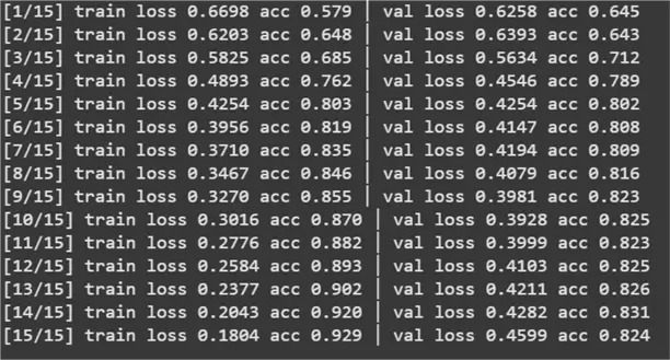
We have achieved impressive results with our model with a final accuracy score of 82.4%. Recall that the RNN on the same dataset achieved an accuracy of 65%. Since we kept the entire model pipeline constant, with the same hyperparameters and dataset, this nearly 17% improvement can be attributed to the BiLSTM network architecture.
Conclusion
In this tip, we have explored and explained the theoretical foundations of the Long Short-Term Memory (LSTM) network. To solidify these concepts further, we used a BiLSTM model to compare our previous approach to sentiment classification with an RNN to highlight the superiority of this architecture.
Next Steps
- Interested readers are advised to understand the inner mechanics of BiLSTMs further to better understand how they were able to outperform our simple vanilla RNNs by a large margin.
- Another route to undertake is to study Gated Recurrent Units (GRUs), a simplified version of LSTMs, that retain similar capabilities but use fewer gates, making them computationally more efficient.
- Finally, learning about sequence-to-sequence models, encoder-decoder architectures, and how LSTMs are used in them (especially in older translation models) will give readers a strong foundation for understanding modern NLP and sequence modeling techniques.
- Check out more AI-related tips.
