Problem
In this series of tips, we will delve into the unsupervised learning branch of Machine Learning. Principal Component Analysis (PCA) is a powerful technique for dimensionality reduction, but its mathematical foundation involving eigenvalues and eigenvectors can be intimidating. This tip aims to demystify PCA, explaining its purpose, how it works, and its use in visualizing high-dimensional data.
Solution
With most real-world problems, data is often collected containing a huge number of features. Think of:
- MNIST dataset containing hundreds of pixel values.
- Medical record-based datasets containing large numbers of indicators for individuals’ health.
- Economics datasets containing features spanning across time, as well as across different entities.
The examples are endless. While there may be a general belief that more features equate to a better model performance after training, this is generally not true. Thus, Principal Component Analysis (PCA) is a vital tool that enables us to condense a dataset with numerous features into a smaller dataset with fewer features while still retaining important patterns from the original dataset.
The Need for PCA
So why are more features not always beneficial?
Reduce Dimensionality
In high-dimensional settings, more features usually create more problems than help as data becomes sparse. For example, in 2D, you might need a few hundred points to cover a space, but in 100D, you need an astronomical number of points to make a cluster. Such problems are often attributed to the curse of dimensionality.
Many ML algorithms, such as KNN, require the assumption that data points are close together for the model to yield accurate results. However, in a high-dimensional dataset, these points appear far apart, and distance metrics, like Euclidean distance, lose meaning as the difference between the nearest and farthest points becomes negligible. This can cause the KNN model to break down in a high-dimensional space.
This concept is illustrated in the diagram below. We can observe a dataset of six observations somewhat uniformly spread across a 1D space, 2D space, and 3D space, all with the same unit size. It is rather immediately clear that although the points are quite close together in the 1D space, they become farther apart in the 2D space, and even more sparse in the 3D space. Therefore, PCA can be a vital tool in reducing the dimensionality of datasets, so models, like KNN, that require spatial closeness of data points, can work optimally.
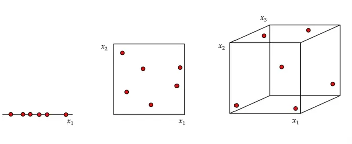
We can easily extrapolate the concept of the diagram above to a real dataset with millions of data points and thousands of variables. Despite such an enormous number of observations, these data points will be extremely sparse in a thousand-dimensional space if they are assumed to be uniformly spread.
Preserve Underlying Structure
Unfortunately, we cannot illustrate such a dataset to highlight the sparsity. This brings us to our second crucial point. We humans can only visualize data up to the 3-dimensional space. However, we will rarely find a dataset with only three features. Therefore, for pattern recognition, exploratory data analysis, or stakeholder communication, it is helpful to project data into 2D or 3D using PCA while preserving as much of its underlying structure.
Identify Uncorrelated Underlying Features
Moving on, there are other ML models, like linear regression, that assume the features are independent of each other. However, in many datasets, some features are redundant and correlated with other features, which can bias the model’s weights and predictions. For instance, think of a dataset with features, such as the number of heat strokes, forest fires, sales of ice cream, units of ACs bought, and so on. However, if we think for a bit, all of these variables are highly correlated with each other and thus redundant, as the underlying temperature variable can explain them all. In such cases, PCA can help identify uncorrelated underlying features like temperature.
Identify Noisy Features
In an equivalent manner, data with a large number of features are more prone to model overfitting. More features can lead to more complex models, which may memorize training data instead of learning general patterns. Especially when the number of features is greater than the number of observations, models tend to fit to noise in the dataset. This ultimately leads to a weaker model performance. PCA helps to identify these noisy features.
Keep Costs Down
Lastly, another obvious reason we want to avoid is the high computational complexity cost that comes with it. More features equate to more memory requirements, longer training, and inference times, which can reduce scalability and efficiency of our ML models.
Thus, PCA is a very flexible and robust tool that can be applied to a range of problems caused by a high-dimensional dataset.
Basics of Linear Algebra
Now that we have a good understanding of why PCA is a necessary technique to learn, it is equally important that we shed some light on its mathematics before we fully explore its algorithm. At its core, PCA relies heavily on concepts from linear algebra. Let’s take a look at some of the key concepts below:
Vectors and Matrices
A vector is simply an ordered list of numbers and can be thought of as a point or a direction in space. An example of a position vector  is shown below:
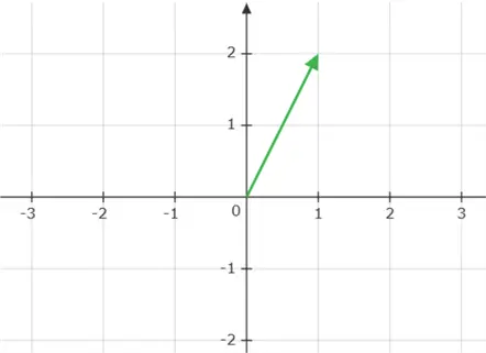
In PCA, a single data point is usually represented as a vector. For example, a dataset with 3 features can represent each observation as a 3-dimensional vector.
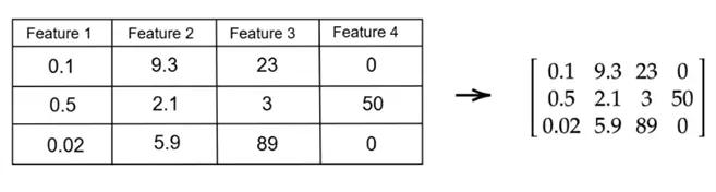
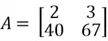
As you are already familiar with, a matrix is a rectangular array of numbers, typically used to represent a dataset (with rows as data points and columns as features) in the context of PCA. If you have a dataset with  rows and
  features, your dataset can be represented as a matrix of size
  as shown below:
A matrix is called a square matrix if it has the same number of rows and columns.
Scaling
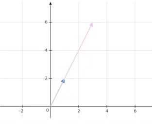
Vectors can be scaled to change their magnitude by multiplying them by a scalar. Consider the same vector as before: . If  is multiplied by 3 as shown below, its magnitude will triple while the direction it is pointing to remains unchanged.
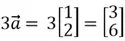
This is also illustrated graphically below:
If the value of the scalar lies between 0 and 1, the vector will shrink while pointing in the same direction. If it lies between -1 and 0, the vector will again shrink, but its direction will reverse. As an example, if is multiplied by -0.5, we get the following results:
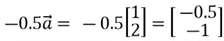
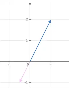
Similarly, if the value of scalar is less than -1, the vector will scale up on its magnitude and reverse its direction.
Magnitude of a Vector
The magnitude of a vector measures how long the vector is in space. For a vector  of size
  , its magnitude can be computed as follows:
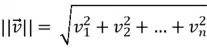
It tells you the distance of the vector from the origin.
Transpose
Transpose is a simple operator that flips a matrix over its diagonal, by which the rows and columns are exchanged. It is easily below:
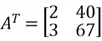
As you can see, the first row becomes the first column, and the second row becomes the second column in the transposed matrix.
Determinant of a Matrix
The determinant of a square matrix is a single number that summarizes certain key properties of that matrix. Although the discussion over these properties will be beyond the scope of this tip, we will still attempt to highlight some of their key characteristics.
Geometrically speaking, the determinant of a square matrix represents the scaling factor of area when the matrix is applied as a linear transformation. To calculate the determinant of a square matrix of size 2, we can use the following formula:
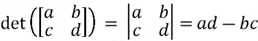
For square matrices of other sizes, different numerical methods exist, as it is very tedious to produce them manually otherwise.
If the determinant of the covariance matrix is zero, it means one or more features are perfectly linearly dependent, and the data lies in a lower-dimensional subspace. PCA helps detect and remove these redundancies. This property will be important later.
Dot Product
The dot product of two vectors measures how aligned they are. If the dot product is zero, the vectors are orthogonal or perpendicular to each other. As an example, consider the two position vectors and  below.
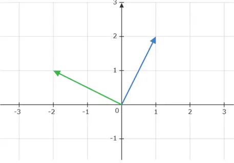
We can observe that these two position vectors are perpendicular to each other. However, to mathematically establish this fact, we need to compute the dot product of these two vectors, which is denoted as:

In short, the dot product is calculated by summing the products of corresponding components of the vectors.
Covariance Matrix
The covariance matrix summarizes the covariances between multiple random variables. For a dataset with n features, its covariance matrix will be a square matrix of size n. The formula used to compute this matrix is as follows:
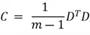 Where
Where  is the number of data points, and
 is our dataset matrix.
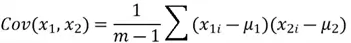
The entries of this covariance matrix reflect the covariance of one variable with every other variable in the dataset. Covariance between two variables can be calculated using the following formula:
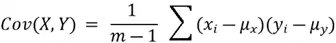
Where is the total number of data points,  is the mean of the
  variable, and
  is the mean of the
  variable.
Consider a dataset with two features: and  . The value of its covariance matrix can be broken down as follows:
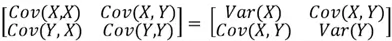
It is important to note here that the covariance of a variable with itself is simply the variance of the said variable. Moreover, covariance is order invariant in the sense that 
Eigenvalues and Eigenvectors
The concepts of eigenvalues and eigenvectors are central to PCA. Given a square matrix  , an eigenvector
  satisfies the following equation:

Where  is the eigenvalue associated with .
In simple terms, eigenvectors are non-zero vectors that, when transformed by a matrix, only change in magnitude, not direction. The amount they are scaled is given by the corresponding eigenvalue, a scalar value. Imagine a matrix as a transformation that can rotate, stretch, or shrink vectors. An eigenvector is a special vector that, when acted upon by this transformation, only gets stretched or shrunk. The eigenvalue represents the factor by which the eigenvector is stretched or shrunk.
How Does PCA Work?
Now that we are covered some of the essential concepts of linear algebra, let’s delve into how PCA works as a tool for dimensionality reduction.
Remember that the goal of the PCA is to preserve as much of the original data’s structure as possible. It does so by extracting new features from the dataset as a linear combination of the dataset’s original features.
At a high level, PCA constructs new dimensions from the dataset, which are referred to as principal components:
- First principal component represents the direction of greatest variability in the dataset.
- The second principal component will be perpendicular to the first principal component and represent the remaining variability.
- The third component will be perpendicular to both the first and second principal components.
This process can continue until the original dimensionality of the dataset is reached. These principal components are essentially new dimensions on which we project the data points from our original dataset. However, since the purpose of PCA is dimensionality reduction, we pick far fewer principal components, much smaller than the original dimensionality of the dataset.
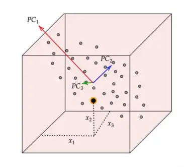
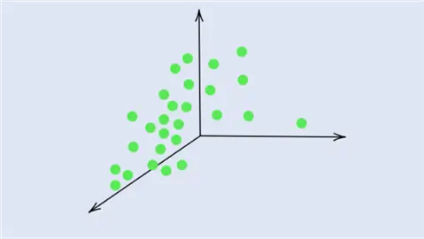
This concept is illustrated in the diagram above. We can observe a 3-dimensional dataset with the original features  and
and  . We can also see that the data has the greatest spread in a diagonal direction from top left to bottom right. This information is encapsulated by the first principal component,
  . The second largest variability in the dataset occurs perpendicular to and this direction is represented by
  . Lastly, the remaining variability in the dataset is captured by the last principal component,
  , perpendicular to all of the PCs.
By picking fewer principal components, most of the dataset’s variability and thus structure is preserved whilst achieving the aim of lowering the dimensionality of the dataset.
Algorithm Behind PCA
So how do we achieve this exactly? While there are several methods of implementing PCA, we will discuss the one that is easiest to understand.
Let us first start with the example dataset shown below:
 |  |
| 4 | 11 |
| 8 | 4 |
| 13 | 5 |
| 7 | 14 |
As you can see, this is a 2-dimensional dataset as it only comprises 2 features. For simplicity, there are a total of 4 data observations. So, to get started, we need to undertake the following steps to implement PCA on this dataset:
- Compute the covariance matrix for this dataset.
- Get the eigenvectors and eigenvalues for the computed covariance matrix.
- Find the first principal component by projecting the data points on the dimension indicated by the first eigenvector.
Since our purpose is to demonstrate dimensionality reduction, we will not calculate the second principal component, as that would just yield the same dataset dimension as our original data. The purpose of PCA is to always find a lesser number of principal components than the number of features in the original dataset.
Let’s start with the first step. Recalling that for the covariance matrix, we need to compute the covariance between  and
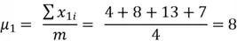
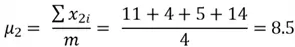
and  , and the variance of both variables. However, first and foremost, we need to calculate the mean of both variables to calculate variance. All these computations are shown below.
First, we get the mean of both variables:
Now we can compute the variance:


We can now move on to computing the covariance between the two features:

Now that we have all of the required values, we can construct our covariance matrix:
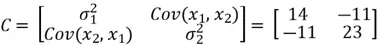
The covariance matrix tells us how features vary with respect to each other. We use it to discover directions in which the data varies the most.
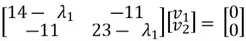
Now we need to calculate the eigenvectors and eigenvalues of our covariance matrix. The eigenvectors tell us about the principal component directions, along which the data varies the most. The eigenvalues indicate the percentage of variance of the data captured in the corresponding direction. This is how we calculate the eigenvectors and eigenvalues using some simple algebra:


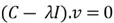
This equation has a non-zero solution if and only if:

We then solve the quadratic equation using the quadratic formula:
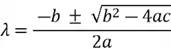
Where 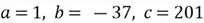 (values from the coefficients of the quadratic equation). Thus:
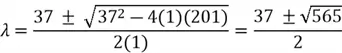
Here,  and
and  represent our eigenvalues. Each of these eigenvalues has its own corresponding eigenvectors.
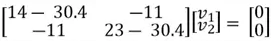
We now need to sort our eigenvalues in descending order and choose the top  eigenvalues and their corresponding eigenvectors. The
 in our case is 1, since we are reducing the dimensionality of the example dataset from 2 to 1. Therefore, since
 , we will select the eigenvector corresponding to as our chosen direction, as it signifies the direction with the most variance.
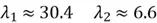
Here is how to calculate the eigenvector  corresponding to :
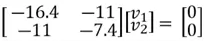
We can then perform matrix multiplication to yield the following set of equations:

We can use the first equation to get:
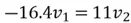
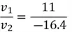
Thus,  , and
, and  and our eigenvector pointing to the direction of maximum variance is
 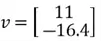 . It is important to note that we can calculate another eigenvector that points in the same direction by using the second equation.
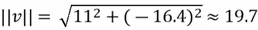
Now that we have our selected eigenvector, it is important to normalize it to ensure that the principal components are comparable and to avoid issues with scaling. In other words, we need to focus on the direction, not the length of the eigenvector. This is done by computing the total magnitude of our eigenvector and dividing each element of the eigenvector by this value:
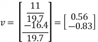
Now, finally, we can find our new extracted features by projecting the original data points on the direction of axes indicated by our selected eigen vector . This is done by simply computing the dot product of each row of the dataset and the eigenvector . However, for this step, it is essential to first de-mean that data as PCA is sensitive to the scale of data.
To accomplish this, we first subtract the mean of both variables from their respective data points:
 |  |
 |  |
 |  |
 |  |
 |  |
This step yields the following dataset:
| |
 |  |
| 0 |  |
 |  |
 |  |
Now we can project each point in the centered dataset onto the first principal component as seen below:
 |
 |
 |
 |
 |
Note how our extracted feature is formed using a linear combination of both of the dataset’s original features. Also, recall that our top highest eigenvalue that we picked had a value of 30.4. This indicates that captures early 30.4% of the variance of the original dataset.
Anyhow, we have successfully implemented dimensionality reduction on our dataset. Suppose if we were working with a larger dataset with multiple features, as is the case in the real world, we would calculate subsequent principal components by again computing the dot product of each row of the dataset with other eigenvectors corresponding to eigenvalues in the chosen top  range.
Implementing PCA in Python
Now that we have the basic understanding of PCA, it is time to further refine this knowledge by implementing PCA practically using Python.
Data Visualization
We will first be demonstrating the use case of PCA for data visualization. For this example, we will use the Iris dataset, which includes measurements of different flower species for classification purposes. This dataset has a dimensionality of 4, and we will reduce it to 2 using PCA to visualize it properly.
Let’s first start by importing the required libraries:
#MSSQLTips.com (Python)
#Importing required libraries
from sklearn.datasets import load_iris
import pandas as pd
from sklearn.decomposition import PCA
import matplotlib.pyplot as plt
Now we can load the dataset:
#MSSQLTips.com (Python)
#load dataset
iris = load_iris()
X = iris.data
y = iris.target
target_names = iris.target_names

iris = pd.DataFrame(iris.data, columns=iris.feature_names)
print(iris.shape)
iris.head()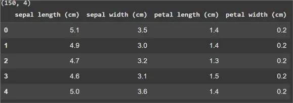
As you can see above, this dataset has 4 features and 150 observations.
Now we can use PCA using the following simple command:
#MSSQLTips.com (Python)
#PCA
pca = PCA(n_components=2)
X_pca = pca.fit_transform(X)
We can now visualize our dataset and inspect the different clusters present:
#MSSQLTips.com (Python)
#Visualization
for target, label in enumerate(target_names):
    plt.scatter(X_pca[y == target, 0], X_pca[y == target, 1], label=label)

plt.xlabel('PC1')
plt.ylabel('PC2')
plt.legend()
plt.title('Iris dataset projected onto first 2 PCs')
plt.show()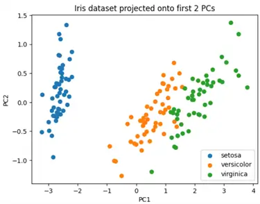
Dimensionality Reduction
We will now use the load_digits dataset to demonstrate how PCA can be used to reduce the number of features in image-based dataset, and reconstruct images from the reduced dimensionality dataset.
First, we need to import the libraries we will need:
#MSSQLTips.com (Python)
#Importing required libraries
from sklearn.datasets import load_digits
import pandas as pd
from sklearn.decomposition import PCA
import matplotlib.pyplot as plt
Now, we load our dataset:
#MSSQLTips.com (Python)
#Load Dataset
digits = load_digits()
X = digits.data

digits = pd.DataFrame(digits.data, columns=digits.feature_names)
print(digits.shape)
digits.head()
Now we can reduce the number of features from 64 to 20:
#MSSQLTips.com (Python)
#PCA
pca = PCA(n_components=20)
X_reduced = pca.fit_transform(X)
X_restored = pca.inverse_transform(X_reduced)
Lastly, we can reconstruct our images and inspect the difference between the original and restored images:
#MSSQLTips.com (Python)
#Show original vs. restored datasets
n = 5
plt.figure(figsize=(10, 4))
for i in range(n):
    # Original
    plt.subplot(2, n, i + 1)
    plt.imshow(X[i].reshape(8, 8), cmap='gray')
    plt.axis('off')
    if i == 2:
      plt.title("Original: 64D")

    # Reconstructed
    plt.subplot(2, n, i + 1 + n)
    plt.imshow(X_restored[i].reshape(8, 8), cmap='gray')
    plt.axis('off')
    if i == 2:
      plt.title("Reconstructed: 20D")


plt.suptitle('Digit Image Compression using PCA', fontsize=14)
plt.tight_layout()
plt.show()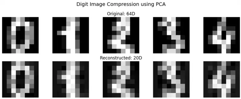
The differences between the two sets of images is indeed negligible despite the decrease in dimensionality!
Conclusion
In this tip, we have successfully introduced Principal Component Analysis (PCA). Readers are first introduced to why PCA is an essential technique in the machine learning domain, followed by a brief introduction to linear algebra and subsequent explanations about the theory and algorithm of PCA. We ended the discussion by demonstrating how PCA can be implemented in Python to visualize high-dimensional datasets or for dimensionality reduction purposes.
Next Steps
- For the more curious readers, they should attempt to employ PCA on the MNIST dataset and see how the performance of a fixed neural network varies between the original dataset and the lower-dimensional dataset. Investigate the performance of the model vs. the time of training utilized.
- Since PCA assumes the underlying subspaces in the dataset to be linear, investigate how non-linear datasets can be transformed before PCA is used on them. Also, try to find out why PCA is not an ideal tool to be used on a dataset for classification.
- Look into concepts related to the direction of class separability and the direction of maximum spread. Research how LDA-Linear Discriminant Analysis might be a better fit for such scenarios.
- Look into other dimensionality reduction techniques for data visualization, such as t-SNE, which is much better at preserving structures within datasets. Look into what the ideal scenarios are where PCA and t-SNE shine the most.
- AI-related tips
