Problem
You have learned about the importance of statistics in a SQL Server database, but you don’t understand it very well. Furthermore, when you learn that the DBCC SHOW_STATISTICS command gives you information about statistics, you execute it and its output adds more confusion. In this tip I will explain how to interpret the outputs of the SQL Server DBCC SHOW_STATISTICS command.
Solution
One of the most misunderstood concepts of Database Administration is statistics and its interpretation. For those of you who don’t know much about the importance of statistics, just to give you an idea, they are a determining factor when the database engine needs to build an execution plan, even more than indexes. In fact, SQL Server will use the available statistics associated with an index to decide if its usage is beneficial. That fact usually causes beginners to confuse both concepts by thinking that statistics are a part of indexes. The relationship between indexes and statistics is not symmetric; every index has statistics associated with it, but not all statistics have a corresponding index.
DBCC SHOW_STATISTICS
DBCC SHOW_STATISTICS shows the actual status for a given statistic on a table or indexed view. The output of this command is composed of three items; the statistic header, the density vector and the histogram. In this tip we will dig into these concepts, but first I will show you the most basic syntax and its output.
DBCC SHOW_STATISTICS(Object_Name, Statistic_Name)
Where Object_Name is the name of the table or indexed view and Statistic_Name is the name of the statistic.

DBCC SHOW_STATISTICS Statistics Header
This item shows the basic information about a statistics.
| Column name | Description |
|---|---|
| Name | The statistics name. |
| Updated | This is the last time the statistics was updated. |
| Rows | This represents the total number of rows of the underlying (a table or indexed view) at the moment when the statistics were last updated. An easy way to see if your statistics are outdated is to compare this number against the actual number of rows. But be aware that if the statistics corresponds to a filtered index then the value of this column is the number of rows that match the filter at the moment when the statistics were last updated. |
| Rows Sampled | The number of rows analyzed to generate the statistics. |
| Steps | This is the number of steps in the histogram. I will go on this topic when I introduce you to the histogram. |
| Density | This item is not used by the query optimizer and is for backwards compatibility only. |
| Average Key Length | The average size in bytes of the column or set of columns that composes the statistics. |
| String Index | This value is set to YES if the statistics contains summarized statistics to improve optimization for predicates in the form of “Where Column LIKE ‘%Value’”. |
| Filter Expression | If the statistics are filtered it shows the filter predicate, otherwise it is set to NULL. |
| Unfiltered Rows | If the statistics are filtered it shows the number of rows in the table before applying the filter. Otherwise this value is equal to Rows. |
DBCC SHOW_STATISTICS Density Vector
The DBCC SHOW_STATISTICS density vector measures the distribution of values. It shows one row for each prefix of columns in the statistics. For example, if the statistics is composed of three columns Col1, Col2, Col3 in that order; then we will have three density vectors: the first will be for column Col1, the second for columns Col1 and Col2 and the last for columns Col1, Col2, Col3.
| Column name | Description |
|---|---|
| All Density | This is a number between 0 and 1.It is defined as 1/n where n is the number of distinct values. The closer that Density is to zero the more unique are the key value, that’s why candidate keys have lower density. |
| Average Length | The average size in bytes of the column or set of columns that composes the statistics. |
| Columns | Names of columns in the prefix for which All density and Average length are displayed. |
Let’s see this with an example. First create a sample database.
USE [master]
GO
CREATE DATABASE [sampleDB]
 CONTAINMENT = NONE
 ON  PRIMARY
( NAME = N'sampleDB', FILENAME = N'C:\MSSQL\sampleDB.mdf' ,
 SIZE = 10240KB , MAXSIZE = UNLIMITED, FILEGROWTH = 1024KB )
 LOG ON
( NAME = N'sampleDB_log', FILENAME = N'C:\MSSQL\sampleDB_log.ldf' ,
SIZE = 10240KB , MAXSIZE = 2048GB , FILEGROWTH = 128MB)
GO
Now we create a very simple table consisting on one identity column “ID” that we define as a Primary Key “PK”and a varchar column “Name” and set up an index “IX_Name” on it.
USE SampleDB
GO
CREATE TABLE SampleTable
    (
      ID INT IDENTITY(1, 1) ,
      Name VARCHAR(50) CONSTRAINT PK PRIMARY KEY CLUSTERED ( ID )
    )
CREATE INDEX IX_Name ON SampleTable (Name)
The next step inserts 2000 rows to the table and updates its statistics. Notice that the rows contain the same value for the column “Name”.
USE SampleDB
GO
INSERT  INTO dbo.SampleTable
        ( Name )
VALUES  ( 'John'
          )
GO 2000
exec sp_updatestats
go
We can see now the statistics on “PK”.
USE SampleDB
GO
DBCC SHOW_STATISTICS('SampleTable','PK')
GO
As you can see on the next image the Density Vector has a density very close to zero because all values of ID column are different.

Let’s do the same, but with the statistics on “IX_Name”.
USE SampleDB
GO
DBCC SHOW_STATISTICS('SampleTable','IX_Name')
GO
The next image shows that the Density Vector for the Name column is equal to 1 because all values are the same.

DBCC SHOW_STATISTICS Histogram
The DBCC SHOW_STATISTICS histogram is a representation of the distribution of values across a fixed number of intervals that can go up to 200. In order to create the histogram the optimizer sorts the column values, then sets limit values that will define the upper bounds of the histogram steps. After this, the optimizer summarizes the values that fit on each step.
| Column name | Description |
|---|---|
| RANGE_HI_KEY | Upper bound column value for a histogram step. The column value is also called a key value. |
| RANGE_ROWS | Estimated number of rows whose column value falls within a histogram step, excluding the upper bound. |
| EQ_ROWS | Estimated number of rows whose column value equals the upper bound of the histogram step. |
| DISTINCT_RANGE_ROWS | Estimated number of rows with a distinct column value within a histogram step, excluding the upper bound. |
| AVG_RANGE_ROWS | Average number of rows with duplicate column values within a histogram step, excluding the upper bound. It is calculated by dividing RANGE_ROWS by DISTINCT_RANGE_ROWS when DISTINCT_RANGE_ROWS is greater than zero, otherwise its value is 1. |
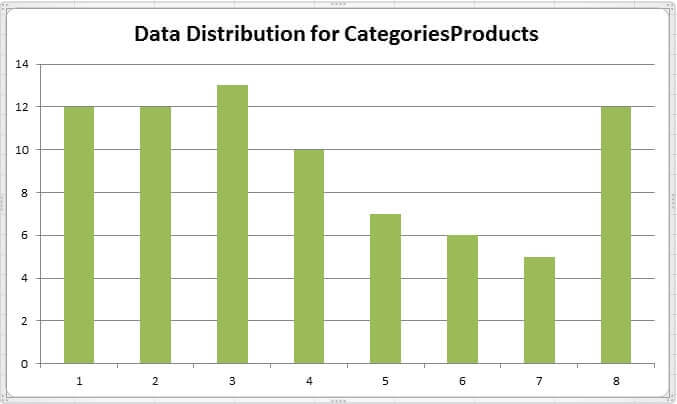
Something you can do with the histogram is to create an Excel graphic, mostly for learning purposes. The next image is a graphic of the data distribution on the Products table from the Northwind database made with the histogram of the CategoriesProducts statistics. The x axis represents a value for column CategoryID of Northwind’s Products table and the y axis is the number of occurrences of that value.
Effects of Statistics on Plan Generation
Let’s do a simple test on the AdventureWorks database. Consider the Person.Person table and the IX_Person_LastName_FirstName_MiddleName statistics histogram.
USE AdventureWorks2012
GO
DBCC SHOW_STATISTICS('Person.Person','IX_Person_LastName_FirstName_MiddleName') WITH HISTOGRAM
GO
If you take a look at its histogram you can see that it has 199 steps. Consider the steps 1, 12 and 13 with keys “Abbas”, “Ashe” and “Bailey” respectively.

Just like I did with the Northwind’s Products table I created a graphic of the data distribution. Also I marked in black the interval of values we are working with.

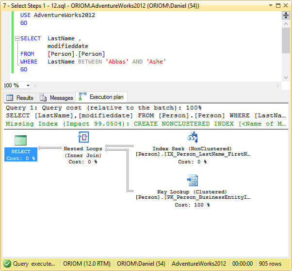
Now we are going to execute a simple select statement on the table to list the persons whose last name is between the range “Abbas” and “Ashe”, which is between steps 1 and 12 of the histogram.
USE AdventureWorks2012
GO
SELECT  LastName ,
        modifieddate
FROM    [Person].[Person]
WHERE   LastName BETWEEN 'Abbas' AND 'Ashe'
GO
We can see on the image below the execution plan of the previous query. The query optimizer decided that an index seek and a key lookup is the best plan.
In the other hand, if we execute the same query, but this time listing the persons whose last name is between the range “Abbas” and “Bailey”, just one step further on the upper boundary.
USE AdventureWorks2012
GO
SELECT  LastName ,
        modifieddate
FROM    [Person].[Person]
WHERE   LastName BETWEEN 'Abbas' AND 'Bailey'
GO
As you can see on the next image, now the query optimizer has decided that the best approach is to perform a clustered index scan.

This effect on plan generation is known as Parameter Sniffing. You can read more about this topic on my previous tip Different Approaches to Correct SQL Server Parameter Sniffing.
Next Steps
- You can download a copy of the AdventureWorks and the Northwind Databases as well as other test databases.
- Need to insert 2000 equal rows in one execution? Read this tip: Executing a TSQL batch multiple times using GO.
- In this tip you will learn how to keep your database statistics up to date. Execute UPDATE STATISTICS for all SQL Server Databases.
- You can get more information about the implications of statistics on plan generation in this tip: Issues Caused by Outdated Statistics in SQL Server.
- Take a look at this tip to learn how SQL Server Auto Update and Auto Create Statistics Options work. After reading the tip you may be able to answer the following question: What are the SQL Server _WA_Sys… statistics? if you can’t, don’t worry. Here is the answer: What are the SQL Server _WA_Sys… statistics?.
- You can find more tips about Performance Tuning on Performance Tuning Tips Category.
