By: Siddharth Mehta | Comments (1) | Related: > Python
Problem
The fundamental process in the machine learning development life cycle is identifying the dependent and independent variables for developing a data model. The two basic categories of supervised machine learning are classification and regression.
Regression is arguably the most basic form of machine learning algorithms and suitable for beginners in machine learning. Though it is one of the most basic algorithms for machine learning, it is also one of the modes widely applied machine learning algorithms, with multiple variations of this algorithm. In this tip we will learn how to develop a machine learning model using a linear regression algorithm.
Solution
It is recommended that if you are new to Python or Machine Learning Services in SQL Server 2017, consider reading the Python and SQL Server 2017 Basics tutorial. It is also assumed that you have SQL Server 2017, Python and Machine Learning Services installed on your development machine.
The first step for any data science exercise is analyzing sample data and determining fields of interest. So, we need to consider a sample dataset that we will use for this exercise, from which we will predict the output of dependent variable using the independent variable. Data Quality is a crucial factor for data science, for which ETL, MDM and other mechanisms are applied to standardize and cleanse data. As our focus in on learning the machine learning model, so we would consider it as granted that we have access to processed quality data.
The next step in machine learning is exploratory data analysis to identify the independent and dependent variables of interest. Since this is more domain driven, we will take it as granted that independent and dependent variables have already been identified to maintain focus on developing machine learning model.
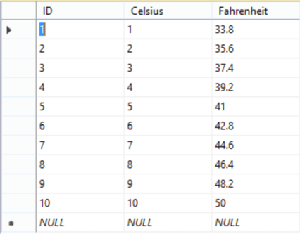
As we have considered the preliminary tasks in machine learning lifecycle as granted, we will be using the dataset as shown below, having just two fields. Generally, after applying techniques like exploratory data analysis, principal component analysis, dimensionality reduction etc., the dependent and independent fields of interest are identified. In the sample dataset of Celsius and Fahrenheit that we are using, consider C as the independent field and F as the dependent or the response field. Our intention is to find the relationship between the two variables from the below dataset.

In real-life scenarios, statistical models would almost never have a perfect linear relationship unless and until it’s a deterministic model. One short-cut method of determining whether linear regression can be applied to the data in question is by creating a scatterplot of dependent versus independent variables and creating a trend line to analyze whether there is a linear or near-linear relationship.
If we create a scatterplot of the data shown above, it would look as shown in the picture below, which is a strong indicator that linear regression algorithms can be applied on this data.
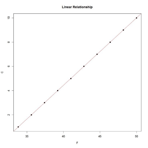
The linear regression algorithm finds the shortest line (also known as best-fit line) that passes through all the data points in a way that all the data points are at a minimum distance from the line. Consider reading more about the statistical formula for this algorithm from here.
We intend to discover the relationship between Celsius and Fahrenheit using linear regression algorithm, and we would implement the same using Python and T-SQL, with the assumption that this data is hosted in SQL Server. Create a table named Readings which has the readings of Celsius and Fahrenheit as shown below before proceeding the actual algorithm implementation.
We will be implementing the T-SQL code for the linear regression algorithm with the approach mentioned below.
- Fahrenheit is the dependent variable and Celsius is the independent variable.
- The formula of ordinary least squares linear regression algorithm is Y (also known as Y-hat) = a + bX, where a is the y-intercept and b is the slope. By applying the algorithm, we will derive the coefficients “a” and “b”.
- In our case, Y-hat is Fahrenheit, X is Celsius, “a” is the Y-intercept and “b” is the slope as shown below. We already know what is X and Y. The result of our model will deliver the values of a and b.
- Using the revoscalepy library we are using functions rx_lin_mod to create linear model and rx_predict to predict Fahrenheit from the linear model.
- Finally, we will print the original input and predicted output in the output data frame.
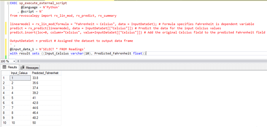
Execute the below code to create a linear model, train the data model using the above dataset and finally predict the output for a given input value.
EXEC sp_execute_external_script
      @language = N'Python'
    , @script = N'
from revoscalepy import rx_lin_mod, rx_predict

linearmodel = rx_lin_mod(formula = "Fahrenheit ~ Celsius", data = InputDataSet); # Formula specifies Fahrenheit is dependent variable and Celsius in independent variable
predict = rx_predict(linearmodel, data = InputDataSet[["Celsius"]]) # Predict the data for the input Celcius values
predict.insert(loc=0, column="Celsius", value=InputDataSet[["Celsius"]]) # Add the original Celcius field to the predicted Fahrenheit field

OutputDataSet = predict # Assigned the dataset to output data frame
' ,
@input_data_1 = N'SELECT * FROM Readings'
Once you execute the above code, the output would look as shown below. From a model life-cycle perspective, we may want to store, extract and use the model at required. For the same we can store the model in a varbinary variable after serializing the model, and deserialize it while extraction. You can learn about this from an example explained in this tip.
We successfully created the model and predicted the output too. But the key value of creating the model is to find the co-efficient values, which gives insights to data analysts or data scientists regarding the influence of independent field on the dependent field. To find out the coefficients “a” and “b”, just print the summary of your linear model, and you should be able to find result as shown below.
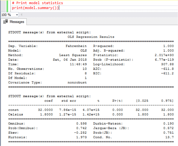
Some points that can be derived from the above result are as follows:
- R-squared is the accuracy of the model with which it was able to explain the variation in the dataset. Here “1” mean 100% variation is explained, so we can be confident that the coefficients are accurate. It is almost never 100% in real-life cases of statistical models.
- There are other statistics as well like skew, kurtosis, p-value, etc. These statistics explain different properties of the model related to accuracy and confidence in the model.
- Using the derived co-efficient and linear regressions equation, we can easily
calculate or predict values. For example, in this case the intercept here is
32 and slope is 1.8. Given that we intend to predict the value of Fahrenheit
for 1 degree Celsius, the formula of linear regression method to predict the
same would be as mentioned below.
Fahrenheit = (Y-intercept) + (slope * Celsius)

i.e. Fahrenheit = 32 + (1.8 * 1) = 33.8.
This means 1 degree Celsius would be 33.8-degree Fahrenheit. Using this equation with the derived coefficients, we can predict the value of Fahrenheit for any given value of Celsius. We have developed a model using Linear Regression algorithm and trained our model by feeding it a dataset, from which it learned and derived inferences to predict intended results. This is what we term as machine learning in its simplest form.
Next Steps
- Consider learning thoroughly about the algorithm of your choice and learn more details of how the implement the same in Python using SQL Server Machine Learning Services.


About the author
 Siddharth Mehta is an Associate Manager with Accenture in the Avanade Division focusing on Business Intelligence.
This author pledges the content of this article is based on professional experience and not AI generated.
View all my tips