Implement Linear Regression in Python for Machine Learning

Problem

Machine learning (ML) often feels overwhelming for beginners, having many complex models and algorithms to grasp. However, at its core, ML starts with simpler techniques, such as the K-nearest neighbor and algorithm and the Naive Bayes classifier. Moving deeper into ML techniques, we now focus on linear regression, one of the most fundamental algorithms, that provides an excellent foundation for understanding more advanced techniques. Additionally in this tip, we will learn how optimization methods like gradient descent and cost functions are crucial for building a strong base in ML along with how to do linear regression with Python.

Solution

Linear regression is perhaps one of the simplest, most commonly used machine algorithms with a wide variety of use cases in business analytics, econometrics, research and development, healthcare—the list goes on. It is a supervised learning algorithm used for predicting a continuous target (dependent) variable based on one or more features or independent variables. Thus, the model assumes linearity in data – if x changes, y is expected to change linearly. The goal of this model is to find the best possible linear relationship between the dependent variable and independent variables.

The model achieves this by fitting a hyperplane in the dataset. A hyperplane is simply defined as a subspace whose dimensionality is one less than its ambient space. So, what do these words mean? Consider the scatterplot below. Its ambient dimensionality is 2, since there are two variables: x and y. A hyperplane in 2-dimensions will thus be 1-dimensional as evidenced by the best fit line, depicted by that dashed blue line. By fitting a straight line through these data points, it attempts to predict outcomes for new data based on this relationship.

Suppose you are a real estate agent and want to build a linear regression model that predicts house prices based on features like crime rate, air quality, property tax, etc. However, for simplicity, you are interested in predicting house prices based on only one feature: the crime rate. This is a simple linear regression setup. So now we have a 2-dimensional dataset, which implies we will have to fit a line through it. In generic terms, the equation of a line can be formulated as:

Where is the predicted value of the house price, and are parameters.

Linear regression is a parametric model. This essentially means that unlike using the entire dataset to predict like we did in K-Nearest Neighbors, we will use a finite number of parameters to make a prediction. In this case, our goal is to find the parameters and (which control the intercept and slope of the line) that best fit a line through the data.

But what if you want to include more features in your regression model? If there are features, our regression equation will look like this:

This is referred to as multivariate linear regression analysis. Here, our ambient dimensionality is , which means our fitted hyperplane will have a dimension of . For example, if we incorporate two features (crime rate and property tax) for our house price prediction, the fitting hyperplane will be 2-dimensional. Here is what the best fitted hyperplane might look:

But the important question is how do we even figure out the parameters Bi that result in the best fitted hyperplane? For this, we need to crack two more puzzles: cost functions and gradient descent.

Cost Functions

To determine how well our linear regression model performs, we need a way to measure its accuracy. Recall that in classification models, accuracy was very easy to define in terms of the total predictions the model got correctly. However, in regression models, the same methodology doesn’t make sense. Suppose that the actual price of a house is but our model predicts the price as . Although the difference is only a dollar, our traditional accuracy formula will completely ignore how close the model’s answer is. Therefore, we need to formulate a new method of accuracy that measures the deviation of the model’s prediction from the actual output. This method should indicate a lower model performance if the deviation is large, and a better performance if the deviation is smaller.

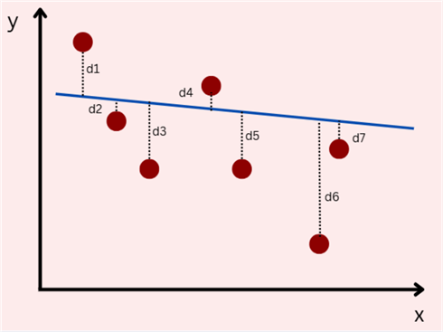
Returning to a simple linear regression case, consider the scatterplot below with a fitted line. For each data point, we measured its deviation from the fitted line. Since deviation is essentially the difference between the actual output and the predicted value by the fitted line, we can define it as follows:

Using this formula, we can infer that if a data point is above the fitted line, the deviation will be positive, but if the point is below the line, the deviation will be negative. This concept will be important later.

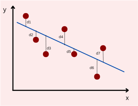
Another deviation in a simple linear regression

Now, for the same dataset, consider the scatter plot below with another fitted line. Visually, it is very clear that this fitted line is much better than the previous one. But, when working with multivariate linear regression, it becomes an unfortunate fact that we cannot visualize more than 3-dimensions. Therefore, we must mathematically establish which fitted line is better.

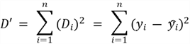
Focusing on the deviations for this plot, we see that they are much smaller than in the previous plot. To quantify this mathematically, we can perhaps sum up the deviations for each data point:

We are expecting that a better fitted line will have a smaller sum of deviations. However, this has a minor problem. Recall that the deviation can both be positive and negative. Therefore, when we are summing all of them, the positives can cancel out the negatives. To deal with this problem, we can simply square the individual deviations:

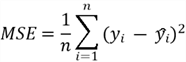
This formula that we have derived is called the square error. If we divide this formula with the number of data points in the dataset, we get the mean squared error (MSE):

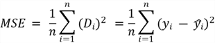
The smaller the MSE, the better our fitted line. This intuitively makes sense: if MSE is small, it has to be because the difference between the fitted line and data points is small. Therefore, for our second plot above, the MSE is likely to be smaller than the first plot.

For this tip, we will be using the MSE metric to evaluate the performance of our regression model due to its simplicity and intuitiveness. Note: Several other metrics like root mean square error (RMSE), mean absolute error (MAE), and Mean Absolute Percentage Error (MAPE) also exist to compare different fitted hyperplanes.

Gradient Descent

Although we have managed to derive a mechanism that helps to identify the better fitted line, we still need a tool that propagates the errors back to the parameters of our hyperplane. So, if our MSE is turning out high, we should be able to alter our parameters that reduce the error. For this purpose, we have the gradient descent algorithm–an amazing iterative optimization technique that allows us to train our models with the objective of minimizing the error.

Our goal is to find parameters that minimize our objective function, which is MSE in this case. For beginners, gradient descent can seem complex, but it boils down to adjusting the model parameters based on how steeply the error decreases with each iteration. Think of the cost function as a mountain, where the height of each point represents the amount of error in the model’s predictions. The goal of gradient descent is to descend the mountain to find the lowest possible point, where the error is minimized. Just as you would take steps downhill based on how steep the slope is, gradient descent takes steps in the direction that reduces the error.

To measure the slope of our mountain, the MSE function, we need to measure its slope with respect to the parameters, or take the derivative, which tells us the direction and steepness of the slope. The steeper the slope, the bigger the steps gradient descent will take, moving quickly towards the minimum. To break down this concept, let’s consider the figure below:

Suppose that our function MSE looks like the parabola above when plotted against the parameter.formula The goal of the gradient descent algorithm is to reach point , where the error is minimized and the gradient is zero. At point , the gradient of the function is negative (as increases, MSE decreases). This gradient remains negative for all values to the left of point . In this region, we want the value to increase to reach the minimum point. At point however, the gradient is positive (as increases, MSE increases). For any value of to the right of point , the gradient will remain positive, and we would want the value to decrease to reach the optimal point .

In short, there are two important observations:

For a negative gradient, we should increase the value of .
For a positive gradient, we should decrease the value of .

Now that we have all the requisite knowledge, here is the gradient descent algorithm:

We randomly initialize the parameters of our model.
The gradient of the cost function with respect to parameters is then computed. Through calculus, the gradients can be computed as:

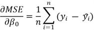
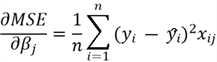
Once we have these gradients, we can update the parameters using the following formula:

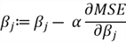
Note that if the gradient is negative, we will be adding to the value of and thus increasing it. If the gradient is positive, we will be subtracting from the , and thus decreasing it.

here is the learning rate. It is a hyperparameter that controls the size of the step we are taking towards the minimum of our MSE function. If is very small, it will take very long to reach the minimum point. On the other hand, if is very large, we can potentially miss the minimum and fail to converge. Therefore, we need to find an appropriate value for through hyperparameter tuning.

We repeat steps 2 and 3 until the MSE stabilizes and does not decrease much further.

For simplicity, we will employ the batch gradient descent technique in this assignment where gradients with respect to the parameters are computed for the entire training dataset in each iteration. Other methods can include stochastic gradient descent and mini-batch gradient descent. Also, note that the algorithm mentioned above is a very basic version of gradient descent. Practically, some advanced variations of the algorithm are employed which are significantly faster.

The Algorithm of Linear Regression

Now that we have all the tools in place, it is time to formally define the linear regression algorithm:

Define the model equation: This process involves identifying the relevant features in your dataset, and establishing the following equation:

Define the Cost Function: To find the best-fit line, we need a way to measure how well our model fits the data. For this purpose, we will be using MSE:

Apply Gradient Descent to Minimize the Cost Function: We will optimize our cost function to find the model parameters that yield the smallest MSE on the training dataset. For each parameter, the update rule is:

Make Predictions: Once we have identified the best fitting hyperplane for our dataset, we can use it to predict our test dataset and evaluate the performance again using MSE.

Implementing Linear Regression in Python

Now that we understand the nuts and bolts of linear regression, it is time for a more practical demonstration. We will be doing that by implementing the algorithm from scratch, as well as by Sklearn on the Boston House Prices. Our goal here will be to implement a multivariate linear regression model that can predict house prices with reasonable accuracy.

Our first step would be to import the following libraries:

#MSSQLTips.com
import numpy as np
import pandas as pd
import matplotlib.pyplot as plt

Now we can start loading the dataset. There are a total of 13 features like per capita crime rate, nitric oxide concentration, property tax rate, number of rooms, river proximity, etc. Our dependent variable is the median house value.

#MSSQLTips.com
X_train = pd.read_csv("/content/data/trainData.txt", sep=" ", header=None)
Y_train = pd.read_csv("/content/data/trainLabels.txt", sep=" ", header=None)
X_test = pd.read_csv("/content/data/testData.txt", sep=" ", header=None)
Y_test = pd.read_csv("/content/data/testLabels.txt", sep=" ", header=None)
print("Shape of X_train: ", X_train.shape)
print("Shape of Y_train: ", Y_train.shape)
print("Shape of X_test: ", X_test.shape)
print("Shape of Y_test: ", Y_test.shape)

We can also see a total of 404 observations in the training dataset, and 102 observations in the test dataset. We will now convert our dataset to NumPy for its ease of use later on.

#MSSQLTips.com
X_train = X_train.to_numpy()
Y_train = Y_train.to_numpy()
X_test = X_test.to_numpy()
Y_test = Y_test.to_numpy()
Y_train = Y_train.reshape(-1)
Y_test = Y_test.reshape(-1)

Now we are left with the last important tasks for our data preprocessing, where we standardize our numerical features using the statistics from the training dataset. We will calculate the mean and standard deviation of the features in the training dataset and standardize both training and test numerical features with these stats. We do not use the test data statistics for standardization because we want the unseen data points to adapt to the training data distribution. The purpose of a test set is to simulate new, unseen data. Standardizing it based on its own statistics makes the evaluation less representative of how the model would perform on truly unseen data.

#MSSQLTips.com
def standardize(data):
    mean = np.mean(X_train, axis=0)
    std = np.std(X_train, axis=0)
    return (data - mean) / std
X_train = standardize(X_train)
X_test = standardize(X_test)

Moving on, we can now get to the important part of the implementation. Our task now is to implement the algorithmic steps outlined in the previous section. As shown below, this involves identifying the model equation, the cost function, the derivatives of the cost function, and the gradient descent algorithm.

#MSSQLTips.com
def equation(data_x, beta, b0):
    return np.dot(data_x, beta) + b0
 
def mse(yhat, ytrue):
    return np.mean((yhat - ytrue) ** 2)
 
def gradient_descent(data_x, data_y, beta, b0, learning_rate, epochs):
    loss_data = []
    m = data_x.shape[0]
    for epoch in range(epochs):
        yhat = equation(data_x, beta, b0)
        loss = mse(yhat, data_y)
        loss_data.append(loss)
 
        if epoch % 100 == 0:
            print(f"Epoch {epoch}: Loss = {loss}")
 
        error = yhat - data_y
        db = (1 / m) * np.dot(data_x.T, error)
        db0 = (1 / m) * np.sum(error)
        beta  = beta - (learning_rate * db)
        b0 = b0 - (learning_rate * db0)
    return beta, b0, loss_data

We can now randomly initialize our parameters and pass them on for gradient descent.

#MSSQLTips.com
r_b = np.random.rand(X_train.shape[1]) 
r_b0 = np.random.rand(1)
beta, b0, loss = gradient_descent(X_train, Y_train, r_b, r_b0, 0.01, 1000)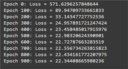

If we plot the loss for each iteration, we can observe a very smoothly decreasing curve. This is a good sign when we are training a model.

#MSSQLTips.com
plt.plot(range(len(loss)), loss, color='red')
plt.xlabel("Iterations")
plt.ylabel("Cost")
plt.title("Trend of Cost over Iterations")
plt.grid(True)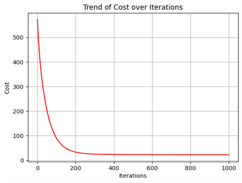

Plot of cost decreasing per each iteration

If we were to predict our test dataset using the parameters we have learned through gradient descent, we will observe a very reasonable model performance.

#MSSQLTips.com
pred = equation(X_test, beta, b0)
testmse = mse(pred, Y_test)
print(testmse)

On the other hand, if we want to avoid implementing everything from scratch, we can use the linear regression module from the Sklearn library to do everything for us in very few lines of code.

#MSSQLTips.com
from sklearn.linear_model import LinearRegression
from sklearn.metrics import mean_squared_error
sklearn_reg = LinearRegression()
sklearn_reg.fit(X_train, Y_train)
y_test_pred = sklearn_reg.predict(X_test)
testmse = mean_squared_error(Y_test, y_test_pred)
print(testmse)

Conclusion

In this tip, we have reviewed and extensively explained the theory behind linear regression. To supplement our explanation, we also focused on an intuitive explanation of cost functions and gradient descent algorithms. We then used a real-world housing price dataset and implemented our very own model from scratch for predictive analysis. Interested readers are also advised to probe further advanced topics in this domain.

Next Steps

Since linear regression requires data to be linear, what can we do if the data is non-linear? Apart from using other non-linear models, it is still possible to use linear regression. Readers can look into data transformation techniques, like log transformation, that can linearize non-linear trends. Another way is to include non-linear variable terms as your features. For example, we can include square terms, interaction terms, square root terms, etc. This type of regression is called polynomial regression.
Another very important concept in linear regression is that of regularization. Techniques like lasso, ridge, and elastic net regularization help the model avoid overfitting the data. Readers are recommended to see how this technique is implemented and how it modifies the gradients and cost function. Furthermore, as mentioned before, different types of cost functions and gradient descent algorithms should also reviewed.
Lastly, readers are strongly suggested to investigate the role of categorical features in linear regression. For this model, incorporating categorical features in regression models requires specific techniques to convert them into numerical forms while preserving information and minimizing distortion. Readers can research methods like dummy coding, one hot encoding, etc.
To checkout more AI related tips.

Resources

Community

Subscribe