Problem
Many companies are leveraging data lakes to manage both structured and unstructured data. However, not all users are familiar with Python and the PySpark module. How can users with a solid understanding of ANSI SQL be effective in the Databricks environment?
Solution
The SQL warehouse in the Databricks ecosystem was released to public preview in November 2020. Please see the release notes for details. The image below shows the components that are part of this offering. One requirement for the warehouse is to have the input data stored as files within Azure Storage. Otherwise, any extract, translate, and load (ETL) operations will be performed with another tool, such as Azure Data Factory Pipeline or Spark Notebook code.

Business Problem
Our manager has asked us to investigate how to leverage the SQL Warehouse to manage our Databricks files. During our exploration, we will cover the following topics:
| Task Id | Description |
|---|---|
| 1 | Warehouse computing |
| 2 | Attach storage to warehouse |
| 3 | Manage existing schemas |
| 4 | Explore DDL statements |
| 5 | Execute DML statements |
| 6 | Identity column behavior |
| 7 | Loading tables |
| 8 | Visuals and dashboards |
| 9 | Scheduling queries |
| 10 | Alerting on query output |
At the end of this article, the data engineer will have a working knowledge of the Databricks SQL Warehouse.
Warehouse Computing
All the menu options for managing our Databrick SQL Warehouse are available under the section called “SQL“. The image below shows there are no existing warehouses under the sub-menu named “SQL Warehouses“.
Let us create a new warehouse now.

There are two cluster scaling concepts to consider when dealing with big data: scale-up (vertical) and scale out (horizontal). Unlike Spark clusters, cluster configuration and size are predetermined in the warehouse. This is sometimes called T-SHIRT sizes since there is a fixed number of choices. Going from an extra small to small cluster size is considered scaling up. The same virtual machine nodes are given more power (CPU + RAM). The cluster scaling section in the image below refers to the number of clusters. Thus, we have the same cluster configuration but duplicate the number of clusters by scaling factor from x (min) to y (max). If the scaling minimum is set equal to the scaling maximum such as a value of two, we are doubling the computing capacity. This feature is considered scaling out.

If we click Create, the warehouse will be deployed. The image below shows a warehouse named “whs-mssqltips-demos“.
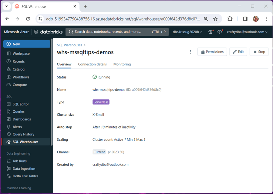
Working in the Azure Databricks Workspace is nice. However, the end users might be familiar with a reporting tool such as Tableau or Power BI. How can we connect those tools to the endpoint? The Connection details tab shows a JDBC string that can be used with Python. Both the JDBC and ODBC drivers can be downloaded from the Databricks website.

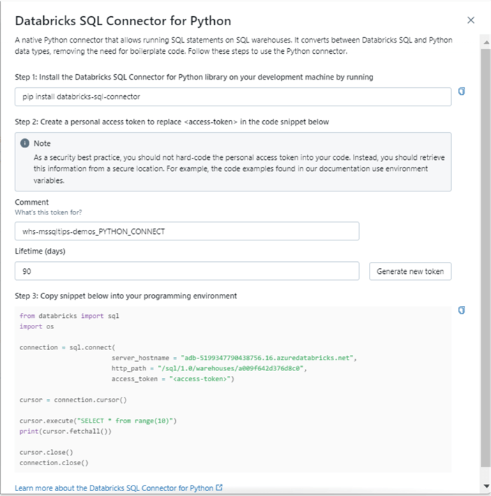
If you click on the product image such as Python, you can get details on how to connect. The image below shows the details about writing a Python program using the Databricks SQL Connect library.
To recap, creating and connecting to an Azure Databricks SQL Warehouse is quite easy.
Attaching Storage
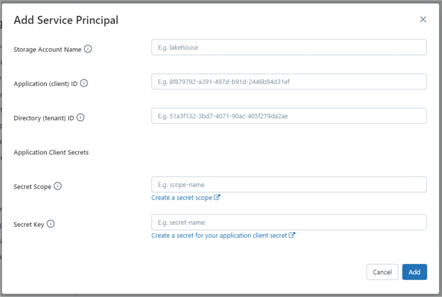
The warehouse uses the Delta Table format. Inserting data one record at a time is not the most efficient way to load data. A better solution is to mount the Azure Data Lake Storage to the Databricks SQL Warehouse. The COPY INTO statement can be used to load files into an existing table. To do this, we need to modify the workspace settings. This task requires a tenant id, service principle, service principal password, storage account URL, and granting access to the data lake storage for the service principle. Only the service principal password is something we do not want to share. This can be locked down using a Databricks Secret Scope that is backed by an Azure Key Vault. See the documentation for details.
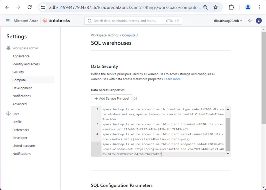
The above image shows the dialog box to enter the data. The image below shows the results after adding our configuration to the Spark cluster for the storage account named “sa4adls2030“.
In a nutshell, Spark is used behind the scenes to execute any SQL queries.
Deleting Schemas
At the heart of both the Spark and Warehouse clusters is the concept of a schema (database). When tables are created, they are published in the hive meta store. Today, we want to clear out some old proof of concept schemas. The DROP SCHEMA statement can be used to perform this work. See the image below for details.

I purposely entered a bug in the Spark SQL statement. There is a misspelling of the word CASCADE. Please fix and re-run the code.

The graphical user interface (GUI) can execute all lines or a given highlighted block of code. The image below shows that the MSSQLTIPS2 schema has been dropped.

To summarize, schemas in Spark are like databases in SQL Server. The tables and views live inside that logical container. If you are not using Unity Catalog, the fully qualified table name is {catalog}.{schema}.{table} with the catalog defaulting to hive_metastore. With Unity Catalog, the default catalog is replaced with the actual catalog name.
Creating Schemas
In the previous section, I skipped over that we were using the SQL Editor menu choice. Any saved Spark SQL code will show up as a file under the Queries menu selection.

I labeled the queries using numbering at the front of the file. Thus, the queries show up in the correct order. The next set of code that we will be exploring is named “01 – Basic Features“. It is very important to know the run-time of a given query so that we can optimize it. The Query History menu option shows recently executed queries. The removal of the MSSQLTIPS2 schema took 721 milliseconds to execute.

One nice feature of Spark schemas is the fact that comments and properties can be associated with the object. The comment is used to give a high-level description of the container. Many data cataloging tools will read and capture this important data. Additionally, the properties section of the schema allows for custom key value pairs. In the example below, I am capturing the user who created the schema and when the schema was created. Please see the CREATE and ALTER schema statements for details.

The image below shows an empty hive schema called adbsql. Let us work on adding tables and data to this schema in the next section.

Exploring DDL Statements
Here, we will create a sample database that shows automobile purchases by country and continent. It is simplistic in nature, but is good enough to express key points about this offering. The code snippet below uses the CREATE TABLE statement to define the ADBSQL.CONTINENT object.
--
-- 1 - create table - continent
--

-- make table
CREATE TABLE
(
  CONTINENT_ID STRING NOT NULL,
  CONTINENT_NAME STRING
);

-- show details
DESCRIBE TABLE EXTENDED ADBSQL.CONTINENT;
We can execute an INSERT INTO statement to add seven rows of data to the table. Please see the snippet below for details.
--
-- 2 - load table - continent
--

-- add data
INSERT INTO ADBSQL.CONTINENT VALUES
    ('A', 'Africa'),
    ('B', 'Asia'),
    ('C', 'Europe'),
    ('D', 'North America'),
    ('E', 'South America'),
    ('F', 'Oceania'),
    ('G', 'Antarctica');

-- show data
SELECT * FROM ADBSQL.CONTINENT;
The image below shows the output from executing a SELECT statement.

The complete code and sample data will be enclosed at the end of the article as a zip file. To shorten the article, I will skip redundant tasks. The next step creates and loads data into a table named ADBSQL.CARS_BY_COUNTRY. The output from a simple SELECT statement is show below.

We can create a SELECT statement that LEFT JOINS the CARS to the CONTINENTS. The image below shows the first six rows. The Databricks SQL Warehouse supports many types of joins. I suggest reading a prior article for more details.

For repetitive SQL statements, it might save the end user coding time by creating a view. The CREATE VIEW statement below returns all columns from the CARS table and one column from the CONTINENT table.
--
-- 3 - Create view for previous query
--

-- make view
CREATE VIEW ADBSQL.CAR_DATA
AS
SELECT
    A.*, B.CONTINENT_NAME
FROM
    ADBSQL.CARS_BY_COUNTRY AS A
LEFT JOIN
    ADBSQL.CONTINENT AS B
ON
    A.CONTINENT_ID = B.CONTINENT_ID;

-- show data
SELECT * FROM ADBSQL.CAR_DATA;
The SHOW TABLES statement shows both views and tables regardless of their state (static or temporary).

The data definition language (DDL) statements start with the keywords CREATE, ALTER, or DROP. They are used to create objects in the database.
Execute DML Statements
Having a static table is very boring. Therefore, the ANSI SQL designers came up with the data manipulation language (DML). The INSERT, SELECT, UPDATE, and DELETE statements are typically nicknamed CRUD. We have some new car data from Greenland. Let’s see if a row exists in the CARS_BY_COUNTRY table using a SELECT statement.

Since data does not exist in the table, we can use the INSERT statement to add a row of data. Note: The raw results show how many rows are affected and the row action.

Only CHECK CONSTRAINTS are supported in a workspace that does not have Unity Catalog enabled. If Unity Catalog is enabled, we can add both PRIMARY and FOREIGN KEY CONSTRAINTS. I have added a check constraint and this insertion of a percent change greater than 100 percent has violated that check constraint.

We found out that the data engineer had the wrong information when writing the query. The image below shows an UPDATE statement with a percentage of 10 that does not trigger the check constraint.

Finally, we can remove data from the table using the DELETE statement.

The four standard CRUD statements work as expected in the Azure Databricks SQL Warehouse.
Identity Column Behavior
We can define an emissions id column in our table using the identity feature. The Spark SQL code below creates the ADBSQL.EMISSIONS_BY_COUNTRY table and inserts two rows.
--
-- 4 - caution use of identity column
--

-- make table
CREATE TABLE ADBSQL.EMISSIONS_BY_COUNTRY
(
  EMISSIONS_ID BIGINT GENERATED ALWAYS AS IDENTITY (START WITH 1 INCREMENT BY 1),
  COUNTRY_ID SMALLINT NOT NULL,
  EMISSIONS_YEAR INT,
  EMISSIONS_AMT BIGINT
);

-- fake data
INSERT INTO ADBSQL.EMISSIONS_BY_COUNTRY (COUNTRY_ID, EMISSIONS_YEAR, EMISSIONS_AMT)
  VALUES (1, 2022, 100);

-- fake data 1
INSERT INTO ADBSQL.EMISSIONS_BY_COUNTRY (COUNTRY_ID, EMISSIONS_YEAR, EMISSIONS_AMT)
  VALUES (2, 2022, 200);
The expected results are shown below.

We can use the DELETE statement to remove all rows. Then re-execute the INSERT statements. Just like T-SQL, the identity column is not reset to 1.

We can use the TRUNCATE statement to remove all rows. Then re-execute the INSERT statements. Unlike T-SQL, the identity column is not reset to 1.

Only the CREATE OR REPLACE TABLE statement will fix this issue. By replacing the table, we reset the identity value in the hive meta store. The TRUNCATE statement does not perform this action.

In short, the TRUNCATE statement does not work like T-SQL. Other than that, the identity column is a nice way to add a surrogate key to a table.
Loading Tables
In this section, we will talk about weak file formats and strong file formats. Additionally, we’ll discuss what is an unmanaged table and a managed table. The comma separated values (CSV) format is considered a weak format since we must infer the schema, column names are optional, and compression is not built in. At the start of the article, we connected storage to the warehouse. Now we are going to use that connection to create tables.

The above image shows all the CSV files from the Adventure Works (Sales LT) database. The code below uses the LOCATION option to place a hive table over the CSV file. This is an unmanaged table; it does not support database properties such as INSERT, UPDATE, and DELETE. Dropping an unmanaged table only updates the hive table. The existing files in data lake storage still exist.
--
-- 5 - Currency - Dataset
--

-- remove table
DROP TABLE IF EXISTS ADVWRKS2.DIM_CURRENCY;

-- create external table
CREATE TABLE ADVWRKS2.DIM_CURRENCY
(
  CurrencyKey INT,
  CurrencyAlternateKey STRING,
  CurrencyName STRING
)
USING CSV
LOCATION 'abfss://sc4adls2030@sa4adls2030.dfs.core.windows.net/bronze/saleslt/csv-files/DimCurrency.csv'
OPTIONS
(
    header = "false",
    delimiter = "|"
);

-- show dataset
SELECT * FROM ADVWRKS2.DIM_CURRENCY;

-- show table
DESCRIBE TABLE EXTENDED ADVWRKS2.DIM_CURRENCY;
The output from the query shown below is the first five rows of the dim_currency table in the advwrks2 schema.

Typically, the output from a Spark job is a directory with one or more files. The Apache Parquet file format is considered strong since it is binary, strongly typed, and supports compression. The image below shows a directory for each table in the AdventureWorks database.

The Spark SQL code below drops an existing table, creates a new empty table, and copies data into the table while merging the schema. This table supports ACID properties of a database. However, it still is an unmanaged table.
--
-- 6 - Currency - Dataset
--

-- remove table
DROP TABLE IF EXISTS ADVWRKS1.DIM_CURRENCY;

-- create table (no schema)
CREATE TABLE IF NOT EXISTS ADVWRKS1.DIM_CURRENCY
USING DELTA
LOCATION 'abfss://sc4adls2030@sa4adls2030.dfs.core.windows.net/silver/saleslt/DimCurrency.delta';

-- copy into (merge schema)
COPY INTO ADVWRKS1.DIM_CURRENCY
FROM 'abfss://sc4adls2030@sa4adls2030.dfs.core.windows.net/bronze/saleslt/parquet-files/DimCurrency/'
FILEFORMAT = PARQUET
COPY_OPTIONS ('mergeSchema' = 'true');

-- show - Dataset
SELECT * FROM ADVWRKS1.DIM_CURRENCY;

-- show table
DESCRIBE TABLE ADVWRKS1.DIM_CURRENCY;
The output from the query shown below is the first five rows of the dim_currency table in the advwrks1 schema.

There are many ways to load data, and we explored two ways to complete that task. Testing is vital to any programming process. The image below shows the final record counts by table. This should be compared to the source files for accuracy.

Visuals and Dashboards
Report designers like denormalized views while database designers like normalized tables. Let us create a view named “ADVWRKS1.RPT_PREPARED_DATA” that flattens several tables. We are interested in sales by year, region, and product.
--
-- 7 - Create a view
--

CREATE OR REPLACE VIEW ADVWRKS1.RPT_PREPARED_DATA
AS
SELECT
   pc.EnglishProductCategoryName
  ,Coalesce(p.ModelName, p.EnglishProductName) AS Model
  ,c.CustomerKey
  ,s.SalesTerritoryGroup AS Region
  ,c.BirthDate
  ,months_between(current_date(), c.BirthDate) / 12 AS Age
  ,CASE
      WHEN c.YearlyIncome < 40000 THEN 'Low'
      WHEN c.YearlyIncome > 60000 THEN 'High'
      ELSE 'Moderate'
  END AS IncomeGroup
  ,d.CalendarYear
  ,d.FiscalYear
  ,d.MonthNumberOfYear AS Month
  ,f.SalesOrderNumber AS OrderNumber
  ,f.SalesOrderLineNumber AS LineNumber
  ,f.OrderQuantity AS Quantity
  ,f.ExtendedAmount AS Amount
FROM
  ADVWRKS1.fact_internet_sales as f
INNER JOIN
  ADVWRKS1.dim_date as d
ON
  f.OrderDateKey = d.DateKey

INNER JOIN
  ADVWRKS1.dim_product as p
ON
  f.ProductKey = p.ProductKey

INNER JOIN
  ADVWRKS1.dim_product_subcategory as psc
ON
  p.ProductSubcategoryKey = psc.ProductSubcategoryKey

INNER JOIN
  ADVWRKS1.dim_product_category as pc
ON
  psc.ProductCategoryKey = pc.ProductCategoryKey

INNER JOIN
  ADVWRKS1.dim_customer as c
ON
  f.CustomerKey = c.CustomerKey

INNER JOIN
  ADVWRKS1.dim_geography as g
ON
  c.GeographyKey = g.GeographyKey

INNER JOIN
  ADVWRKS1.dim_sales_territory as s
ON
  g.SalesTerritoryKey = s.SalesTerritoryKey;
Execute the above Spark SQL to create the view. The output of selecting from the view is shown below.

Currently, our manager is interested in aggregated data: total products sold by region/year and total sales sold by region/year.
--
-- 8 - Use view in aggregation
--

SELECT
  CalendarYear as RptYear,
  Region as RptRegion,
  SUM(Quantity) as TotalQty,
  SUM(Amount) as TotalAmt
FROM
  ADVWRKS1.RPT_PREPARED_DATA
GROUP BY
  CalendarYear,
  Region
ORDER BY
  CalendarYear,
  Region;
The raw output shown below was produced by executing the above Spark SQL.

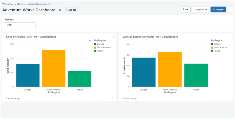
We can use a parameter to pick the year that we want. The image below shows the two bar charts and the raw results as output.

We can pin each chart on a dashboard for a quick report that management can view.
In a nutshell, the Databricks SQL Warehouse does support reporting. However, it is not as sophisticated as other cloud products.
Scheduling Queries
To demonstrate alerts, we need data that is changing in our warehouse. The Spark SQL below creates a CAR_MILEAGE table if it does not exist, inserts a new record, and displays that record.
--
-- 9A - create table (one time), add new row, and show new row
--

-- make table?
CREATE TABLE IF NOT EXISTS ADBSQL.CAR_MILEAGE
(
  MILEAGE_ID BIGINT GENERATED ALWAYS AS IDENTITY (START WITH 1 INCREMENT BY 1),
  MILEAGE_AMT BIGINT,
  MILEAGE_DT TIMESTAMP,
  COUNTRY_ID SMALLINT NOT NULL
);

-- add new row
INSERT INTO ADBSQL.CAR_MILEAGE
(
  MILEAGE_AMT,
  MILEAGE_DT,
  COUNTRY_ID
)
SELECT CAST(RAND() * 5000000 AS INT) AS MILEAGE_AMT, CURRENT_TIMESTAMP() AS MILEAGE_DT, 1 AS COUNTRY_ID;

-- show new row
SELECT TOP 1 (*) FROM ADBSQL.CAR_MILEAGE ORDER BY MILEAGE_ID DESC;
We can schedule the query to run every minute. This adds a new record on that chosen interval.

That was easy to do. However, this simple schedule opens possibilities we did not have previously. The COPY INTO command can now run on a schedule to refresh the warehouse with new data. In the next section, we will talk about alerting.
Alerting On Query Output
Please do not get confused with the numbering. The enclosed file that contains the code below is called “09 – Alert Query”. In this article, the section of code is labeled 9B. Basically, the query returns TRUE (1) every 5 inserts into the mileage table. All other executions return FALSE (0).
--
-- 9B – return a true or false flag
--

-- notify when max id is divisible by 5
SELECT
    CASE WHEN MOD(MAX(MILEAGE_ID), 5) = 0 THEN 1 ELSE 0 END AS FLAG
FROM
    ADBSQL.CAR_MILEAGE;
The Alerts menu section is where you can create or delete an alert. The trigger condition looks for the FLAG column equal to 1. The alert has its own schedule which can be different that the query that loads the data. We must define the email addresses of who will be notified when the alert is triggered.

The image below shows an alert message sent to “John Miner” as the recipient.

A real use case for alerting can be the monitoring of critical sales events. For instance, I work for a company that sells bikes. If we have zero sales for a given day, then we should be worried since AdventureWorks has both in-person stores and online web shopping. This alert can be scheduled every morning for the prior day’s sales.
Summary
The creation of the Databricks SQL Warehouse service competes for market share with products like Snowflake and Fabric Warehouse. Users familiar with ANSI SQL can be up and running with workloads very quickly. More advanced developers can use Spark to load and transform data. Regardless, once the data is placed into Delta Lake, users can use the warehouse to query data. The visualization and dashboard features can support the end users’ simple reports. Scheduling of queries allows table changes to happen at a given time. Please note that stored procedures and user-defined functions are not supported. Finally, the use of alerts is helpful for end users with processes that might see drastic changes.
To recap, a fully functional warehouse can be created within Databricks SQL Warehouse within minutes. Internal tools like autoloaders can be used to load tables if the files exist in cloud storage. If the files do not exist, Azure Data Factory’s copy activity supports many connectors to move data files.
Remember: A limited number of file formats are supported by Spark. External tools like Fivetran can be used to load the warehouse with data that might be on-premises or in-cloud. The variety of data sources goes up exponentially with external tools. Once the data is in the warehouse, it can be queried by external tools using the SQL endpoint or internally with the workspace interface.
The most important advancement out of this new service was the Photon query engine. This C++ rewrite and redesign of the code allows for blinding query execution. If you are looking for a way to control a data lake using SQL queries, I suggest you look at this product.
As mentioned previously, here is a zip file with all the SQL queries that were reviewed in this article.
Next Steps
- Be on the lookout for these upcoming tips:
- Advanced Data Engineering with Databricks
- What is the Databricks Community Edition?
- Various Databricks Certifications
- Solving problems with Graphframes
- Introduction to ML Flow within Databricks
- Data Governance with Databricks Unity Catalog
