Problem
The core functionality of Apache Spark has support for structured streaming using either a batch or a continuous method. The two most popular sources of input data are data lake files and Kafka events. Check point files in the data lake are used to keep track of what data has been processed to date. Performance issues may arise when a directory contains a substantial number of files. Databricks saw this limitation and created the Auto Loader feature for data lake files. High performance can be achieved in this situation by enabling file notifications at the storage level. Understanding the differences between the two techniques is key as a big data engineer.
Solution
The best way to understand the differences between the two design patterns is to create a simple project. Structured streaming is supported on any Apache Spark platform. Thus, we can stream data using Fabric Lakehouse. However, Auto Loader is only available to Azure Databricks, which is supported by all three cloud vendors.
Business Problem
Our manager has asked us to investigate how to load files into our Delta Lakehouse using both streaming techniques. The following list of tasks will be explored during our investigation.
| Task Id | Description |
|---|---|
| 1 | SQL Tables |
| 2 | JSON Files |
| 3 | Notebook Overview |
| 4 | Data Exploration |
| 5 | Structured Streaming |
| 6 | Autoloader |
At the end of this article, the data engineer will have a working knowledge of the streaming data and be able to schedule those notebooks with workflows.
SQL Tables
Big Jon’s Barbeque is one of our customers that wants to conduct a proof-of-concept for streaming data with Azure Databricks. Customers sign up for a shipment of meat that is delivered monthly. The database schema has the following tables:
- Pig packages – a new package is sent to a customer each month.
- Dates – a table that breaks dates down into various attributes.
- Customers – contact information for the customers as well as the pig package they started with.
A simple rotation of packages ensures that different customers receive different pig parts each month. Please see the ERD diagram below for details.
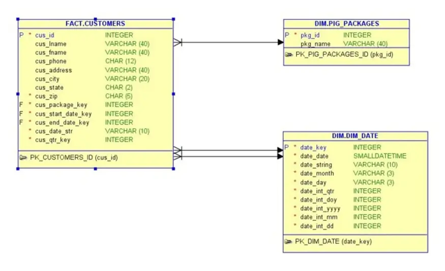
Is this the best design for the database schema? No, it is not. There should be a separation between the customer and sales order header. Additionally, quantity and pricing information should be captured in the sales order detail. However, the database is good enough since the main fact table contains almost one million records.
JSON Files
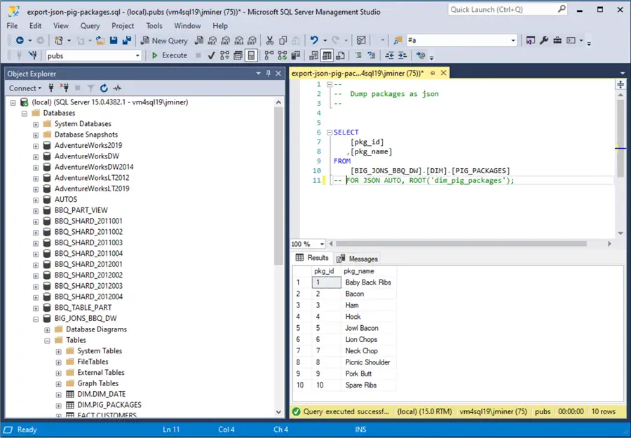
The FOR JSON AUTO ROOT clause of the SQL statement can be used to create an array of JSON records. The image below shows the information displayed in a grid format within SQL Server Management Studio (SSMS).
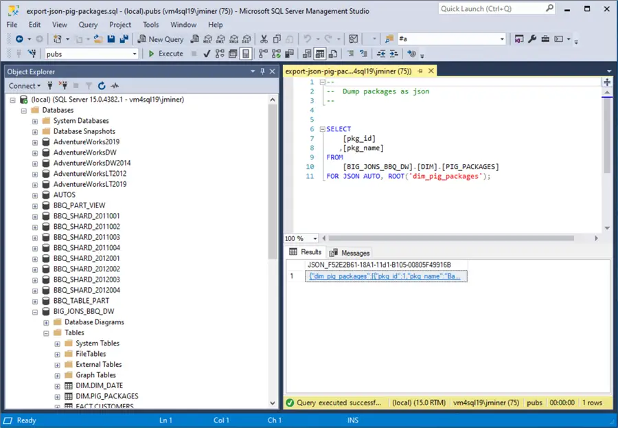
The output shown below is a JSON document representing the table data. For exceedingly small datasets, we can copy the text and save it into a text file to be uploaded into Azure Data Lake Storage. However, for bigger datasets, the following problems might be encountered. The “save as text” option from the results grid inserts carriage returns in the output file. The size of the output is limited by the results in SSMS. I was able to manually save the “dim_pig_packages” and “dim_date” tables as JSON files.
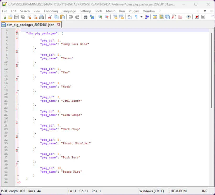
The image below shows the pig packages dataset.
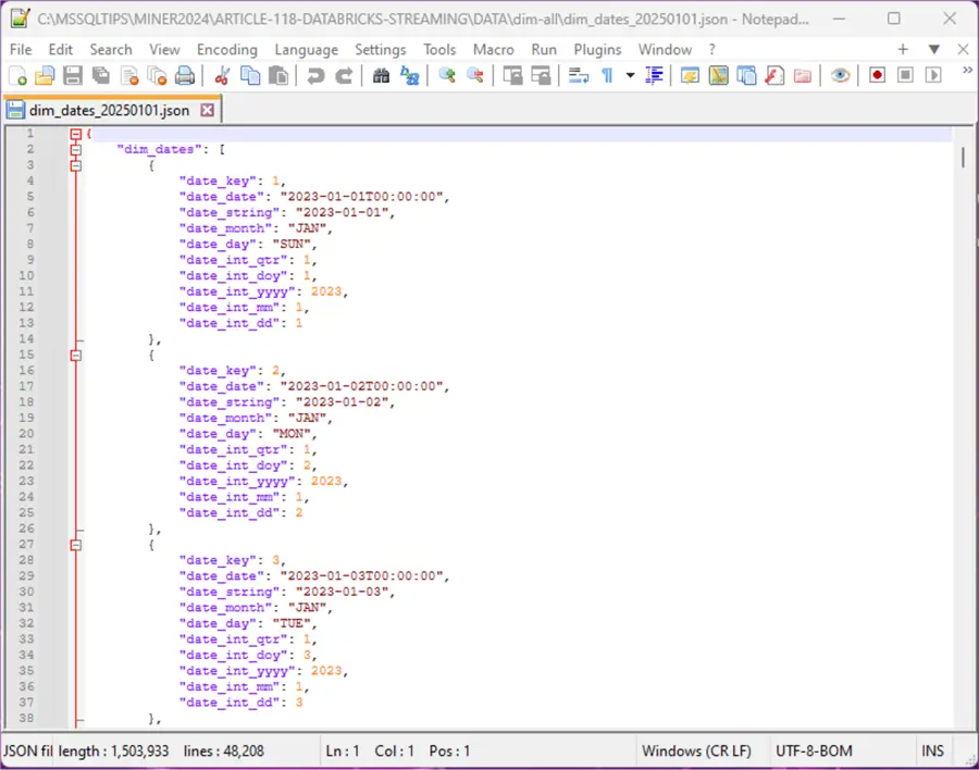
The image below shows the dates dataset.
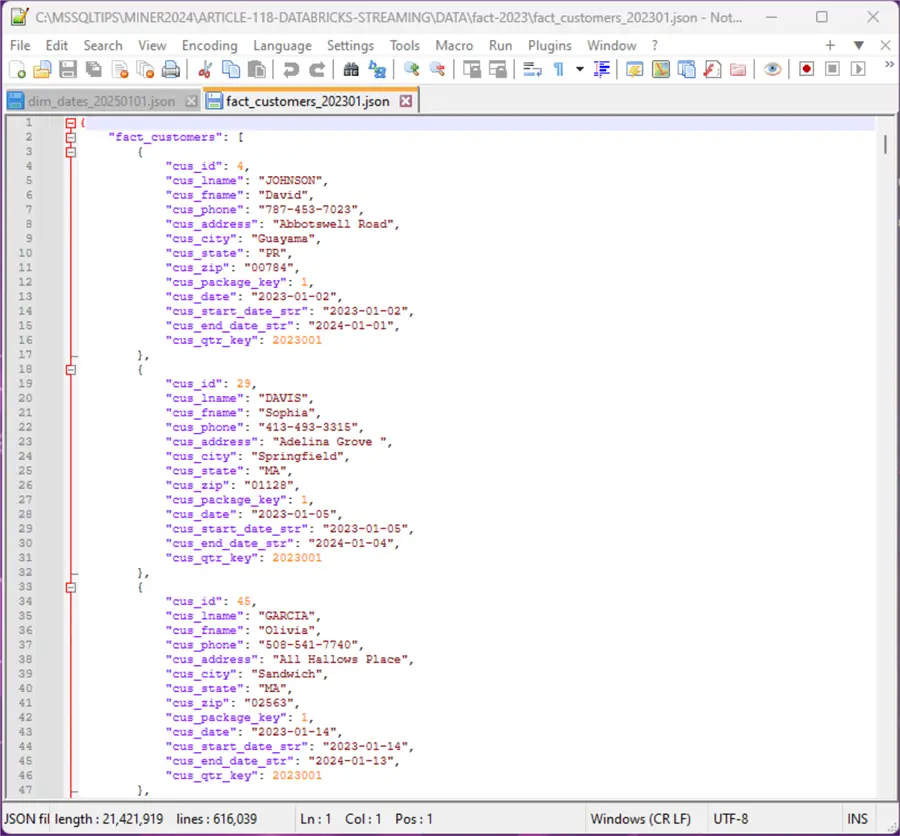
The image below shows the customer dataset for January 2023. As you can see, the JSON format bloats the size of the file. This is not a good format for transferring enormous amounts of data between two systems.
In short, I had to write a PowerShell script that broke down the two years of customer information into 24 files. Explanation of the program is out of scope for this article. However, the code can be downloaded from the provided links at the end of the article.
Load source files into Azure Data Lake Storage
Now that we have our source files, they need to be uploaded into our Azure Data Lake Storage, which is mounted to our Azure Databricks Workspace. The image below shows there is a directory for each of the tables in the bronze medallion zone. Additionally, the parent directory contains the name of the data source since the data lake might contain data from different source systems.

The image below shows the dates JSON file in the correct directory. The JSON file has a sortable date stamp at the end of the file name. Since dimensional data rarely changes, we do not have to create sub-directories to manage large file volumes. The sample data files are enclosed as a download at the end of this article. Please upload these files to your own Azure Storage Container.

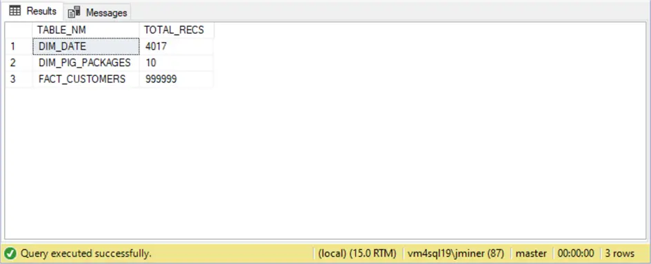
It is always important to capture profile data from the source system. At a minimum, we should check row counts to make sure the data transfer was flawless. Spot checking records and comparing column profiles is another sanity check we can use. The image below shows the row counts that we need to match with our Delta tables in Azure Databricks.
To recap, the creation and staging of JSON files into the bronze medallion zone can be achieved in many ways. Today, we demonstrated that small datasets can be processed by hand. Larger datasets need to be processed with a programming language like PowerShell.
Notebook Overview
The folder below shows the four notebooks that we will be covering in this article.
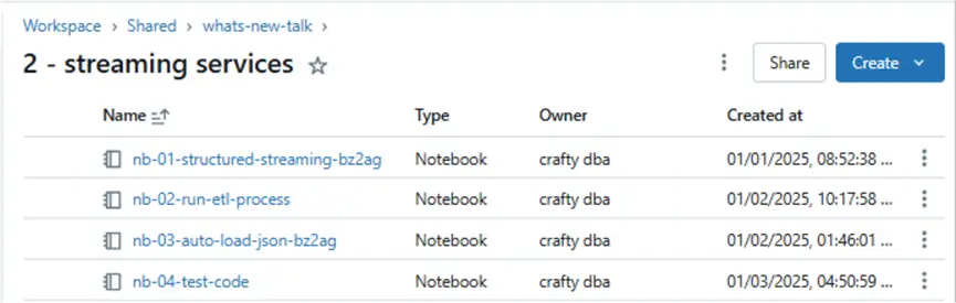
- nb-01-structured-streaming-bz2ag: Demonstrates how to use structured streaming to load JSON files into a Delta table. The code uses the MERGE function of the delta format to provide UPSERT functionality.
- nb-02-run-etl-process: Orchestrates the data loading. The first two cells in this notebook load the pig packages and dates tables using structured streaming. The third cell in the notebook executes the Auto Loader notebook to APPEND data to the final table.
- nb-03-auto-load-json-bz3ag: Demonstrates how to use the Auto Loader feature.
- nb-04-test-code: Demonstrates (explores) how to convert sample JSON into a Spark structure for streaming. Additionally, we want to grab record counts from the Delta tables and compare them to previous ones captured from SQL Server.
Data Exploration
The data structures for JSON files can be quite complex. There is a little know Spark function called schema_of_json that can help. The code below takes the JSON for the “dim_pig_packages” document as input. The output is a string data type.
%sql

--
-- 1 - sample json for dim_pig_packages -> string
--

SELECT schema_of_json('{"dim_pig_packages":[
    {"pkg_id":1,"pkg_name":"Baby Back Ribs"},
    {"pkg_id":2,"pkg_name":"Bacon"},
    {"pkg_id":3,"pkg_name":"Ham"},
    {"pkg_id":4,"pkg_name":"Hock"},
    {"pkg_id":5,"pkg_name":"Jowl Bacon"},
    {"pkg_id":6,"pkg_name":"Lion Chops"},
    {"pkg_id":7,"pkg_name":"Neck Chop"},
    {"pkg_id":8,"pkg_name":"Picnic Shoulder"},
    {"pkg_id":9,"pkg_name":"Pork Butt"},
    {"pkg_id":10,"pkg_name":"Spare Ribs"}
]}') as s
There is an undocumented function that will convert the JSON schema string into a PySpark structure. The code below uses the parse_datatype_string function to end up with a usable PySpark structure.
#
#  2 - convert string into structure
#

# string from previous step
json_schema = "STRUCT<dim_pig_packages: ARRAY<STRUCT<pkg_id: BIGINT, pkg_name: STRING>>>"

# create spark schema
import pyspark.sql.types as t
spark_schema = t._parse_datatype_string(json_schema)
print(spark_schema)
The output below shows a valid PySpark structure that can be used to read in the JSON data file.

Finally, testing is particularly important. The code below gets record counts from Delta tables in the Hive catalog.
%sql

--
--  3 - grab counts by table
--

select 'dim_dates' as table_name, count(*) as total_recs from big_jons_bbq.silver_dim_dates
union
select 'dim_pig_packages' as table_name, count(*) as total_recs from big_jons_bbq.silver_dim_pig_packages
union
select 'fact_customers' as table_name, count(*) as total_recs from big_jons_bbq.silver_fact_customers
Here is the output from executing the above statement:

These counts match the ones captured from SSMS. However, we are putting the chicken before the egg. Let’s start talking about a notebook that uses structured streaming.
Structured Streaming
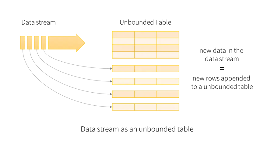
The image below was taken from the Apache Spark documentation on structured streaming. The cool thing about streaming is that we can optionally add additional information to the newly arriving rows before appending them to the final table.
To keep this article manageable, I am going to review the algorithm for the notebook and just cover techniques that are extremely important. The first programming technique is how to use widgets (parameters).
The code below removes all widgets.
#
# Remove all widgets (run 1 time)
#

# dbutils.widgets.removeAll()
The next task is to define the widgets (parameters) used in this notebook.
#
#  Create all widgets
#

dbutils.widgets.text("table_source", "big_jons_bbq.dim.pig_packages")
dbutils.widgets.text("json_schema", "STRUCT<dim_pig_packages: ARRAY<STRUCT<pkg_id: BIGINT, pkg_name: STRING>>>")
dbutils.widgets.text("table_key", "pkg_id")

dbutils.widgets.text("partition_count", "2")
dbutils.widgets.dropdown("debug_flag", "True", ["True", "False"])
dbutils.widgets.dropdown("delete_targets", "True", ["True", "False"])
The next task is to read in the widgets (parameters) and save them as variables for use in the notebook.
#
#  Retrieve all widgets
#


# grab hive catalog vars
source_table = dbutils.widgets.get("table_source")
json_schema = dbutils.widgets.get("json_schema")
table_key = dbutils.widgets.get("table_key")

# grab misc vars
partition = dbutils.widgets.get("partition_count")
debug = dbutils.widgets.get("debug_flag").lower() == "true"
delete = dbutils.widgets.get("delete_targets").lower() == "true"
The power of parameters comes from the fact that we can transform them into new data that is used by the program. First, Azure Databricks without Unity Catalog does not support three dot notations like SQL Server does. Thus, we need to combine the quality zone, source table schema, and source table name as a new Hive table name. Additionally, the JSON structure statement needs to be converted into a Spark SQL statement. This can be done by using the regex library and carefully splitting the data.
#
#  Define variables using widgets
#

# regex library
import re

# create new vars from table info
table_parts = source_table.split(".")
subdir = f"{table_parts[1]}_{table_parts[2]}"
hive_table = f"{table_parts[0]}.silver_{subdir}"
temp_schema = re.sub(r'[<>:]', '', json_schema).split("STRUCT")
table_schema = temp_schema[2]


# create paths to quality zones
bronze_path = f'/mnt/bronze/big_jons_bbq/{subdir}'
silver_path = f'/mnt/silver/big_jons_bbq/{subdir}'
Print statements can be used to see the values stored in the variables. See image below for details.
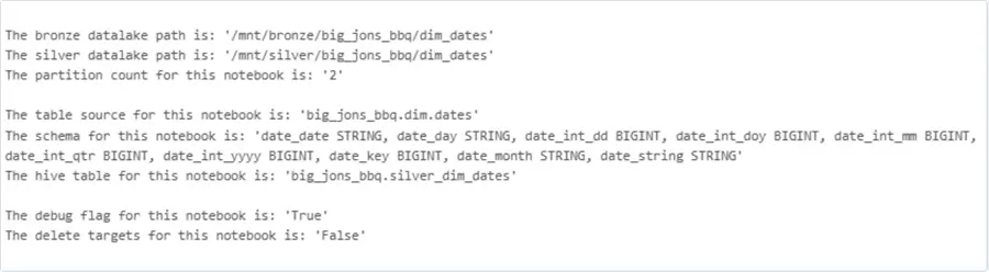
The image below shows how the widgets are defined for the “dim_dates” JSON file. We can easily change the parameters to process the “pig_packages” JSON file.
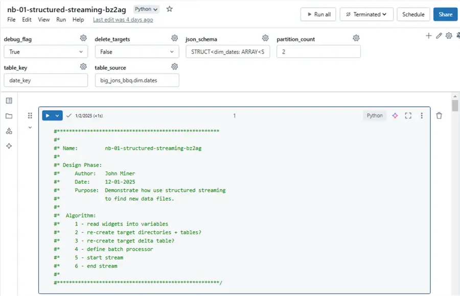
Understanding the process
The image above shows the algorithm used in the notebook. I am going to focus on steps 4 through 6. If we want to rebuild the delta table from scratch, we need to delete and/or drop the target delta table, target delta directory, and target checkpoint directory. If the target table does not exist, we can use the Spark SQL schema to build a brand new empty external delta table.
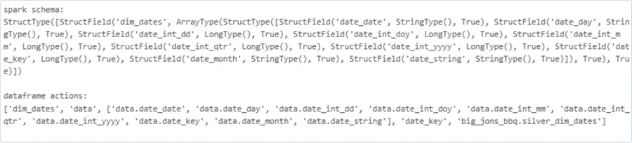
The following actions occur when we use structured streaming: start stream, modify data frame, and end stream. The issue with this pattern is that only one target is allowed, and only appending or overwriting the target is allowed. We can support multiple outputs and different table actions by defining a micro batch processor. Please see the foreachBatch Spark statement for details. Since this is a distributed statement, the global variables defined in the notebook (driver) will not be seen by the executors (workers). There are several solutions to this problem. The easiest is to package the information into a list and pass it as a parameter. I am skipping over the code that does this step. However, the Spark schema and dataframe actions list for the dates dimension is shown below.
A closer look at the code
The first step is to define our micro batch function, which is the most complex piece of code you will see today. We need to use the explode Spark function on the “dim_dates” array to covert the elements into rows within a column named “data”. We want to use the selectExpr to promote each nested column to a main column. Both the load date and source path are added as additional metadata. The withWatermark Spark function allows us to look back in time for late arriving data and the dropDuplicates function prevents errors from occurring during the merge. The DeltaTable.forName Spark function is a nice way to load a table into a dataframe. Finally, we can merge the data on a condition and handle the insert and update actions accordingly.
#
#  Define batch processor
#

# include libraries
from pyspark.sql.functions import *
from delta.tables import *

def process_micro_batch(batch_df, batch_id, input_list):

    # make copy + explode out json
    df_src = batch_df.select(explode(col(input_list[0])).alias(input_list[1]))

    # rename all cols
    df_src = df_src.selectExpr(*input_list[2])

    # add load date
    df_src = df_src.withColumn("_load_date", current_timestamp())

    # add folder_path
    df_src = df_src.withColumn("_source_path", input_file_name())

    # get rid of duplicates
    df_src = df_src.withWatermark("_load_date", "10 minutes").dropDuplicates([f"{input_list[3]}"])

    # Read from disk
    dst_df = DeltaTable.forName(spark, f"{input_list[4]}")

    # create match clause
    match_clause = f"dst1.{input_list[3]} = src1.{input_list[3]}"

    # upsert delta table
    (dst_df.alias("dst1").merge(df_src.alias("src1"), match_clause)
      .whenMatchedUpdateAll()
      .whenNotMatchedInsertAll()
      .execute()
    )
The code to start reading from the stream is simplistic in nature. See the documentation for details on streaming.
#
#  Start stream
#

# set paths
input_path = f"{bronze_path}"
checkpoint_path = f"{silver_path}/checkpoint"

# read in files
df = (spark.readStream
  .schema(spark_schema)
  .option("multiLine", True)
  .option("recursiveFileLookup", "true")
  .json(input_path)
)
The code to start writing the stream to the Hive table involves a lambda function so that we can pass the variables to the micro batch processor. It is important to wait for the stream to terminate if we are just processing files that are available now. The trigger method tells Spark to either run at fixed intervals or consume what data is available now.
#
#  Write stream
#

# write out data
query = (df.writeStream
  .foreachBatch(lambda df, batch_id: process_micro_batch(df, batch_id, input_list))
  .option("checkpointLocation", checkpoint_path)
  .trigger(availableNow=True)
  .start()
)

# await for termination
query.awaitTermination(300)
Did this code work correctly? Of course it did!
Auto Loader
The next two images were copied from the Databricks Engineering blog. The first one shows the main difference between streaming and Auto Loader. While structured streaming can consume both message systems and files, Auto Loader was built for cloud storage.

Typically, structured streaming uses directory listing to discover new files. Auto Loader takes this task to a new level. You can choose to use file notifications at the Azure Storage Services layer or storage directory listing. Even with an incremental listing to reduce the number of inputs, a full listing is taken every eighth time to make sure no files are missed. The “Rocks DB” is a key vault storage unit located in the checkpoint directory. It keeps track of all the files and determines what files are new. The final listing of new files to process is sent over to Apache Spark structured streaming to complete the mission.

The image below shows the widgets being used by the notebook. With the prior structured streaming technique, the table was created first and data was merged into the existing table. With this example of Auto Loader, the Delta table files are appended, and the Hive table is rebuilt at the end of the process.

A closer look at the code
It is apparent that Auto Loader is being used when the format of the data is marked as “cloudFiles.” I am including a link to the documentation for your usage. I will be skipping all variable definitions since they can be found in the notebooks enclosed at the end of the article.
#
# Read files - auto loader
#

# include libraries
from pyspark.sql.functions import *
from delta.tables import *

# read stream
df1 = spark.readStream                                            \
        .format("cloudFiles")                                     \
        .option("cloudFiles.format", "json")                      \
        .option("cloudFiles.inferColumnTypes", "true")            \
        .option("cloudFiles.schemaLocation", schema_path)         \
        .option("cloudFiles.schemaEvolutionMode", "rescue")       \
        .option("multiLine", True)                                \
        .option("recursiveFileLookup", "true")                    \
        .schema(spark_schema)                                     \
        .load(bronze_files_path)
Other than some different options, we are still using the read stream method.
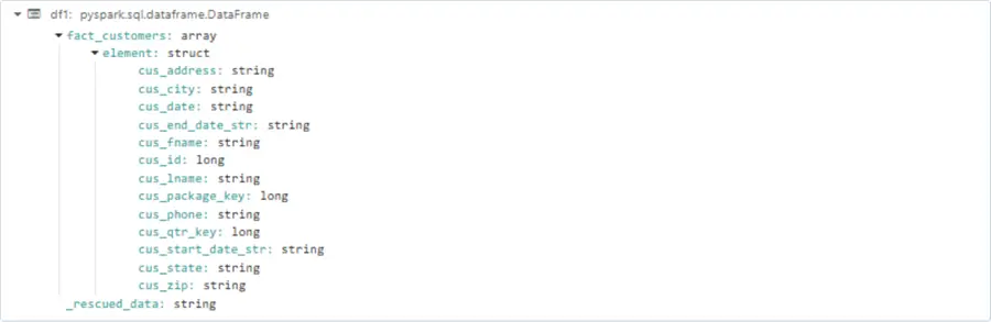
The above image shows the initial resulting dataframe is an array of structures.
#
# Engineer columns - auto loader
#

# make copy + explode out json
df2 = df1.select(explode(col(f"{input_list[0]}")).alias(f"{input_list[1]}"))

# select child nodes
df2 = df2.selectExpr(*input_list[2])

# add date
df2 = df2.withColumn("_load_date", current_timestamp())

# add folder_path
df2 = df2.withColumn("_source_path", input_file_name())
The code to explode and select columns from the dataframe is the same as before. The two additional metadata columns named “_load_date” and “_source_path” are being defined in the output.

The above image shows the resulting dataframe after engineering code is applied as a table with rows and columns.
#
# Write file - auto loader
#

# write delta file
query = df2.writeStream                                    \
        .format("delta")                                   \
        .option("mergeSchema", "true")                     \
        .option("checkpointLocation", checkpoint_path)     \
        .outputMode("append")                              \
        .trigger(availableNow=True)                        \
        .start(silver_files_path)

# await for termination
query.awaitTermination(300)
The output is written to a Delta file format using an append mode. It is especially important to wait for the stream to finish processing. The code below creates the database if it does not exist, drops the existing table, and creates a new external table on top of the Delta files.
#
#   Create missing database, replace existing table def
#

# make sql stmt - create database if not exists
sql_stmt = f"create database if not exists {table_parts[0]}"

# show values
if (debug):
  print(f"The sql statment 1 for this notebook is {sql_stmt}")

# exec sql stmt
df3 = spark.sql(sql_stmt)

# make sql stmt - drop existing hive table
sql_stmt = f"drop table {hive_table};"

# show values
if (debug):
  print(f"The sql statment 2 for this notebook is {sql_stmt}")

# exec sql stmt
df3 = spark.sql(sql_stmt)

# make sql stmt - create new hive table
sql_stmt = f"create table {hive_table} ({table_schema}, `_load_date` timestamp, `_source_path` string) using delta location '{silver_files_path}'"

# show values
if (debug):
  print(f"The sql statment 3 for this notebook is {sql_stmt}")

# exec sql stmt
df3 = spark.sql(sql_stmt)
This is something that I want to explain since I lost several working hours tracking down a bug. One would think that the “create or replace table” syntax would work. For some reason, it results in a table with a messed-up log. Querying the table produces zero records. Querying the parquet files results in the correct number of records. In short, first drop the table and then recreate the table.
Importance of Testing
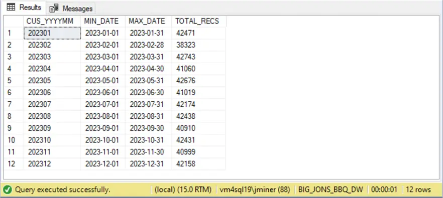
The image below shows the 2023 data by month for the customers fact table.

The Spark SQL code was used to generate the above results from the target system (Spark Delta Tables).
%sql
select _source_path, min(cus_date) as min_date, max(cus_date) as max_date, count(*) as total_recs
from big_jons_bbq.silver_fact_customers
where year(cus_date) = 2023
group by '_source_path'
We now can compare this to the Transact SQL query I ran against the source system (SQL Server Tables).
What I am not showing are the two bugs that I encountered. The first resolved bug was removing the first day of the month due to an equality operator. The second one was that we are using multi-line JSON formatting, which makes the document more readable. However, if we do not supply the correct option to the “spark.readStream” command, we end up with incorrect results. In short, if I had not been diligent in my testing, the bugs would not have been discovered. I have found that testing is an underrated technique I see in the real world today.
Summary
The Azure Databricks service has been around for at least half a decade. During that time, many changes have been made to the product. Initially, to ingest data into a Hive table without worrying about file locations, one used structured streaming. A full directory listing on a folder that has thousands of files can take time. On the other hand, the Auto Loader feature can use file notifications to avoid the pain of performing a complete file listing.
Regardless of technique, check point files are used to keep track of what has been processed. To reload a table from scratch, the Hive table, the Delta file directory, the schema directory, and the checkpoint directory need to be removed. Then recreate the empty directories in the target location and restart the ingestion. I suggest using the Delta file format with streaming since we might want to use advanced operators such as the merge command. Many of the commands I showed today in PySpark code can be done in Spark SQL. However, one must supply all the columns.
The “for each batch” method allows the developer to define custom code for how and where to output the results. Just remember that this function is distributed, and local variables do not work. Passing a list of variables is the most straightforward way to proceed. What I did not show is the fact that one or more outputs can be generated from the stream. Thus, the main table could contain the raw data while the summary table could show aggregates over the batch size. Just remember when re-processing a larger batch of files, duplicates might happen. Therefore, it is important to use the watermark and drop duplicate functions to clean up the data.
Next Steps
Next time, we will be talking about Delta Live Tables (DLT), a declarative framework that can ingest and validate data. This reduces the work that the big data engineer needs to perform by adding structure and limitations to streaming. The DLT coding can be done in both Python and/or Spark SQL.
As previously mentioned, here are three zip files containing the following:
