By: Ron L'Esteve | Comments | Related: > Apache Spark
Problem
Graph Technology enables users to store, manage, and query data in the form of a graph in which entities become vertices and relationships become edges. Graph Analytics enables the capabilities for analyzing deeply grained relationships through queries and algorithms. While many organizations and developers are leveraging graph databases, how can they get started with Graph Analytics by leveraging Apache Spark's GraphFrame API for Big Data graph analysis?
Solution
Apache Spark's GraphFrame API is an Apache Spark package that provides data-frame based graphs through high level APIs in Java, Python, and Scala and includes extended functionality for motif finding, data frame based serialization and highly expressive graph queries. With GraphFrames, you can easily search for patterns within graphs, find important vertices, and more.
In this article, we will explore a practical example of using the GraphFrame API by
- First installing the JAR library,
- Loading new data tables,
- Loading the data to dataframes in a Databricks notebook, and
- Running queries and algorithms using the GraphFrame API.
Before we get started with the demo, lets quickly review some basic graph terminology:
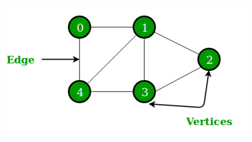
A graph is a set of points, called nodes or vertices, which are interconnected by a set of lines called edges.
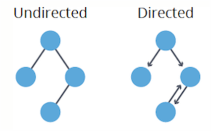
Directed graphs have edges with direction. The edges indicate a one-way relationship, in that each edge can only be traversed in a single direction. A common directed graph is a genealogical tree, which maps the relationship between parents and children.
Undirected graphs have edges with no direction. The edges indicate a two-way relationship, in that each edge can be traversed in both directions. A common undirected graph is the topology of connections in a computer network. The graph is undirected because we can assume that if one device is connected to another, then the second one is also connected to the first:
Install JAR Library
Now that we have a basic understanding of Graphs, let's get started with demonstrating Graph Analytics using the Apache Spark GraphFrame API.
For this demonstration, I have chosen to utilize a Databricks Notebook for running my Graph Analytics, however, I could have just as easily used a Synapse Workspace Notebook, by adding and configuring an Apache Spark job definition in Synapse Analytics and adding the GraphFrame API JAR file to the Spark definition.
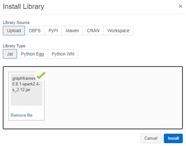
A complete list of compatible GraphFrame version releases can be found here. For this demo, I have used a JAR file for Release Version: 0.8.1-spark2.4-s_2.12 and installed it within the Library of a Standard Cluster.
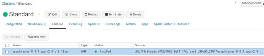
Once the installation is complete, we can see that the JAR is installed on the cluster which will be used to run the Notebook code in the subsequent sections.
Load New Data Tables
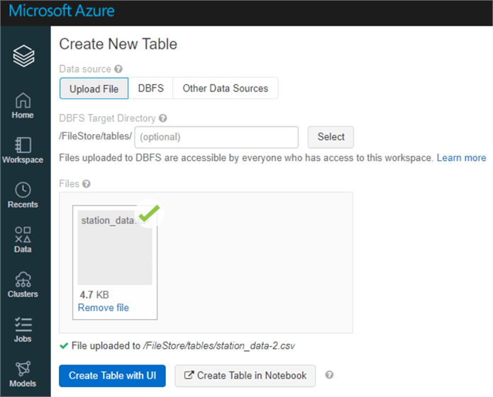
Now that we have the GrapFrameAPI JAR and Cluster ready, lets upload some data via DBFS. For this demo, I will use Chicago CTA Station Data along with Trip Data.
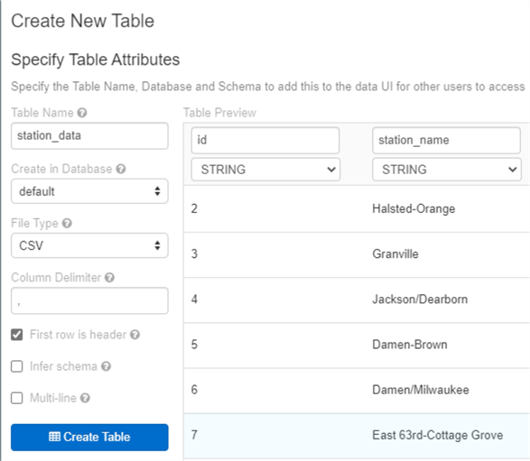
I am creating the station_data table using the UI.
Validate the schema, ensure that 'first row has headers' is checked and create the table.
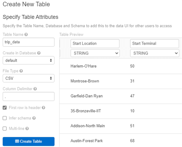
Follow the same process for the trip_data and create the table using the UI.
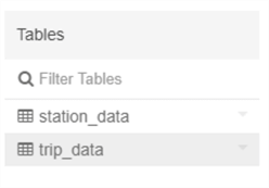
Once the tables are created, they will both appear in the tables section.
Load Data in a Databricks Notebooks
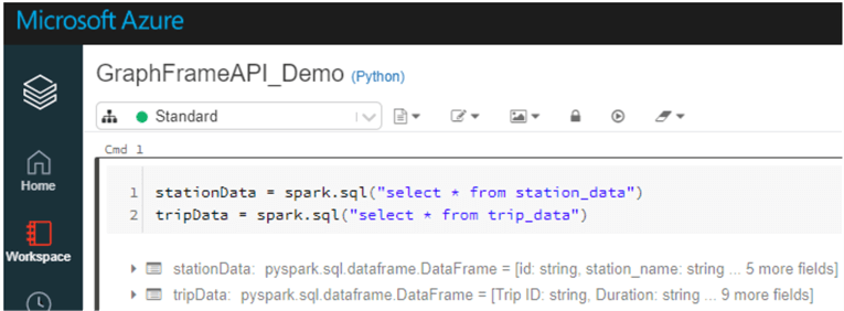
Now that we have created the data tables, let's run the following python code to load the data into two dataframes.
stationData = spark.sql("select * from station_data")
tripData = spark.sql("select * from trip_data")
Build a Graph with Vertices and Edges
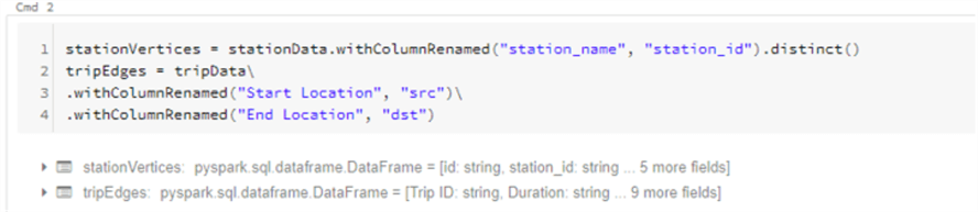
Now that the data is loaded into dataframes, let's define the edges and vertices with the following code. Since we are creating a directed graph, we will define the trips' beginning and end locations.
stationVertices = stationData.withColumnRenamed("station_name", "station_id").distinct()
tripEdges = tripData.withColumnRenamed("Start Location", "src").withColumnRenamed("End Location", "dst")
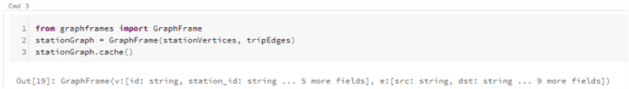
Next, we can run the following code to build a GraphFrame object which will represent our graph using the edge and vertex dataframes we defined earlier. We will also cache the data for quicker access later.
from graphframes import GraphFrame
stationGraph = GraphFrame(stationVertices, tripEdges)
stationGraph.cache()
Query the Graph
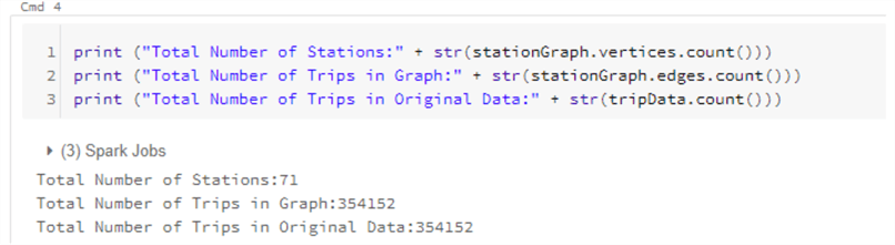
Next, lets run a few basic count queries to determine how much data we are working with.
print ("Total Number of Stations:" + str(stationGraph.vertices.count()))
print ("Total Number of Trips in Graph:" + str(stationGraph.edges.count()))
print ("Total Number of Trips in Original Data:" + str(tripData.count()))
As we can see, there are around 354K trips spanning 71 stations.
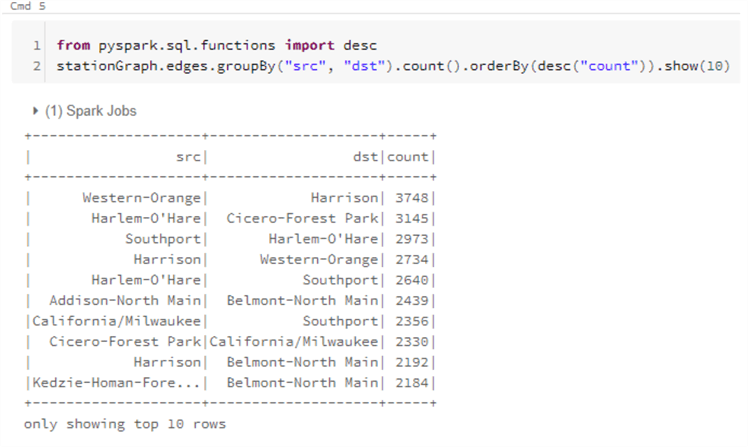
We can run additional queries such as the one below to determine which source and destination had the highest number of trips.
from pyspark.sql.functions import desc
stationGraph.edges.groupBy("src", "dst").count().orderBy(desc("count")).show(10)
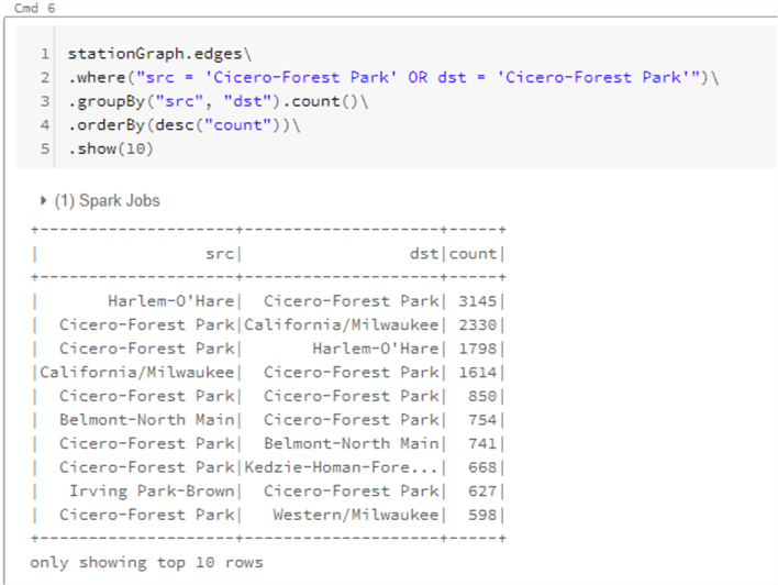
Similarly, we can also run the following query to find the number of trips in and out of a particular station.
stationGraph.edges.where("src = 'Cicero-Forest Park' OR dst = 'Cicero-Forest Park'").groupBy("src", "dst").count().orderBy(desc("count")).show(10)
Find Patterns with Motifs
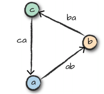
Now that we have run a few basic queries on our Graph data, let's get a little more advanced by finding patterns with something called Motifs which are a way of expressing structural patterns in a graph and querying for patterns in the data instead of actual data. For example, if we are interested in finding all trips in our dataset that form a triangle between three stations, we would use the following "(a)-[ab]->(b); (b)-[bc]->(c); (c)-[ca]->(a)". Basically (a), (b), and (c) represent my vertices and [ab], [bc], [ca] represent my edges that are excluded from the query by using the following operators as an example: (a)-[ab]->(b).
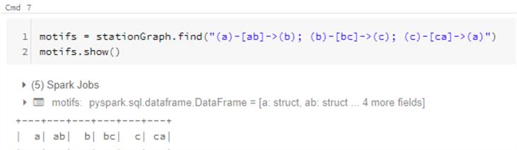
A motif query can be run using custom pattern like the following code block.
motifs = stationGraph.find("(a)-[ab]->(b); (b)-[bc]->(c); (c)-[ca]->(a)")
motifs.show()
Once the motif is added to a dataframe, it can be used in a query as below, for example, to find the shortest time from station (a) to (b) to (c) back to (a) by leveraging the timestamps.
from pyspark.sql.functions import expr
motifs.selectExpr("*",
"to_timestamp(ab.'Start Date', 'MM/dd/yyyy HH:mm') as abStart",
"to_timestamp(bc.'Start Date', 'MM/dd/yyyy HH:mm') as bcStart",
"to_timestamp(ca.'Start Date', 'MM/dd/yyyy HH:mm') as caStart").where("ca.'Station_Name' = bc.'Station_Name'").where("ab.'Station_Name' = bc.'Station_Name'").where("a.id != b.id").where("b.id != c.id").where("abStart < bcStart").where("bcStart < caStart").orderBy(expr("cast(caStart as long) - cast(abStart as long)")).selectExpr("a.id", "b.id", "c.id", "ab.'Start Date'", "ca.'End Date'")
.limit(1).show(1, False)
Discover Importance with Page Rank
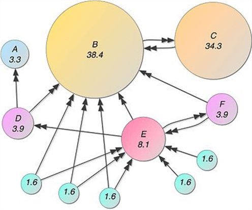
The GraphFrames API also leverages graph theory and algorithms to analyze the data. Page Rank is one such graph algorithm which works by counting the number and quality of links to a page to determine a rough estimate of how important the website is. The underlying assumption is that more important websites are likely to receive more links from other websites.
The concept of PageRank can be applied to our data to get an understanding of train stations that receive a lot of bike traffic. In this example, important stations will be assigned large PageRank values:
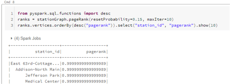
from pyspark.sql.functions import desc
ranks = stationGraph.pageRank(resetProbability=0.15, maxIter=10)
ranks.vertices.orderBy(desc("pagerank")).select("station_id", "pagerank").show(10)
Explore In-Degree and Out-Degree Metrics
Measuring and counting trips in and out of stations might be a necessary task and we can use a metric called in-degree and out-degree for this task. This may be more applicable in the context of social networking where we can find people with more followers (in-degree) than people whom they follow (out-degree).
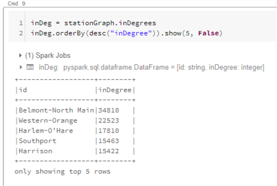
With GraphFrames, we can run the following query to find the in-degrees.
inDeg = stationGraph.inDegrees
inDeg.orderBy(desc("inDegree")).show(5, False)
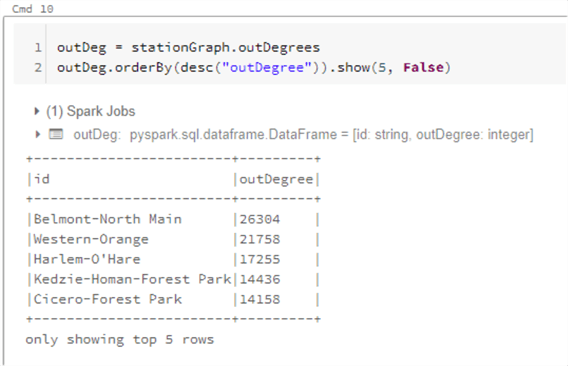
Similarly, we can run the following code to find the out-Degrees.
outDeg = stationGraph.outDegrees
outDeg.orderBy(desc("outDegree")).show(5, False)
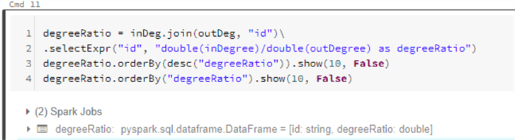
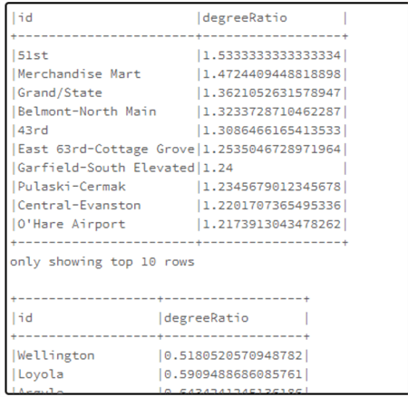
Finally, we can run the following code to find the ratio between in and out degrees. A higher ratio value will tell us where many trips end (but rarely begin), while a lower value tells us where trips often begin (but infrequently end).
degreeRatio = inDeg.join(outDeg, "id").selectExpr("id", "double(inDegree)/double(outDegree) as degreeRatio")
degreeRatio.orderBy(desc("degreeRatio")).show(10, False)
degreeRatio.orderBy("degreeRatio").show(10, False)
Run a Breadth-First Search
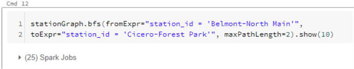
Breadth-first search can be used to connect two sets of nodes, based on the edges in the graph to find the shortest paths to different stations. With maxPathLength, we can specify the max number of edges to connect with specifying an edgeFilter to filter out edges that do not meet a specific requirement.
stationGraph.bfs(fromExpr="station_id = 'Belmont-North Main'",
toExpr="station_id = 'Cicero-Forest Park'", maxPathLength=2).show(10)
Find Connected Components
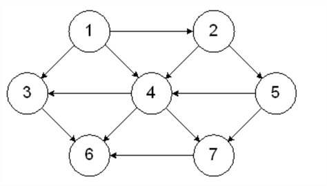
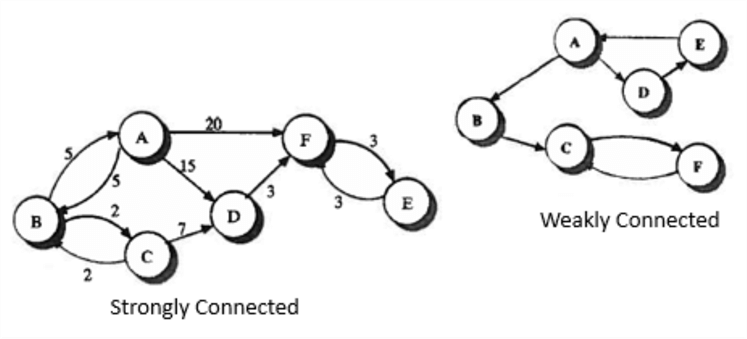
A connected component defines an (undirected) subgraph that has connections to itself but does not connect to the greater graph.
A graph is strongly connected if every pair of vertices in the graph contains a path between each other and a graph is weakly connected if there doesn't exist any path between any two pairs of vertices, as depicted by the two subgraphs below.
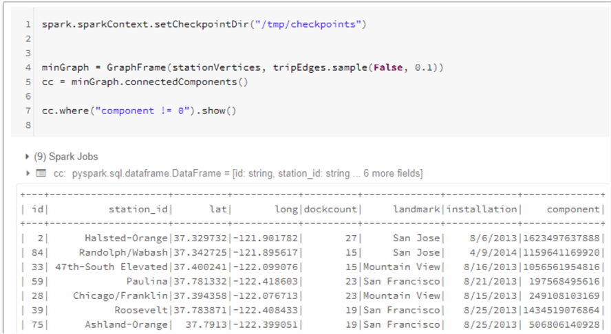
The following code will give us the connected components.
spark.sparkContext.setCheckpointDir("/tmp/checkpoints")


minGraph = GraphFrame(stationVertices, tripEdges.sample(False, 0.1))
cc = minGraph.connectedComponents()

cc.where("component != 0").show()
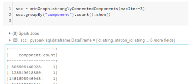
Additionally, we can also find strongly connected components with the following code.
scc = minGraph.stronglyConnectedComponents(maxIter=3)
scc.groupBy("component").count().show()
Next Steps
- Read Spark-The Definitive Guide to Big Data Processing Made Simple
- Learning Spark: Lightning-Fast Data Analytics 2nd Edition
- Read more about Databricks File System (DBFS)
- Read more about Graph Frames in the GraphFrames User Guide
- For more information on DataFrames, read DataFrames tutorial
- For more on Getting started with Apache Spark and Spark packages, read GraphFrames Quick-Start Guide
- For more detail on Spark Pool libraries in Synapse Workspaces, read Add / Manage libraries in Spark Pool After the Deployment
- Explore Supported language and runtime versions for Apache Spark and dependent components
- Read more about graphs in Graph (discrete_mathematics)


About the author
 Ron L'Esteve is a trusted information technology thought leader and professional Author residing in Illinois. He brings over 20 years of IT experience and is well-known for his impactful books and article publications on Data & AI Architecture, Engineering, and Cloud Leadership. Ron completed his Master’s in Business Administration and Finance from Loyola University in Chicago. Ron brings deep tec
This author pledges the content of this article is based on professional experience and not AI generated.
View all my tips