Convolutional Neural Networks for Machine Learning

Problem

Convolutional Neural Networks (CNNs) are highly effective for image processing tasks. However, their layered architecture, including convolutional and pooling layers, can be overwhelming for beginners. This tip simplifies CNNs by focusing on their structure, how they extract features from images and their practical applications.

Solution

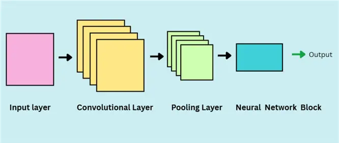
Prior to the advent of large language models (LLMs), Convolutional Neural Networks (CNNs) were the new phenomenal innovations, achieving spectacular results on image classification tasks, which were previously considered to be constricted to human abilities only. For the most part, CNNs are very similar to neural networks – they are also made up of weights with learnable parameters; however, CNNs need to make explicit assumptions about the structure of the input data. It assumes that the data will be image-like, allowing for certain properties to be encoded in the CNN model architecture to specialize in image processing and classification. In the illustration below, you can see a general architecture of a CNN model. The layers shown will be discussed extensively in this tip.

What is an Image?

Before we jump into the nitty-gritty of CNNs, let’s take a detour to define some essential basics first.

You might be wondering how we can classify images in the first place. Well, deep down, images are also numbers! The images that we see on a day-to-day basis on our mobile phones or computers are composed of grids of tiny units called pixels. Each pixel represents the color or intensity of light at a specific point in the image.

Grayscale Images

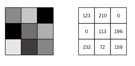
For a grayscale image, like the one shown below, each pixel corresponds to a singular value ranging from 0 to 255, where 0 is black and 255 is white, encoding the intensity and brightness of a particular image. You can observe in the 6×6 pixel image below that darker pixels correspond to smaller values, whereas the whiter pixels have larger values. Moreover, it is also now clear that grayscale images are stored as a two-dimensional array (or a matrix) in a computer’s memory.

Color Images

However, unlike grayscale images, color images, like those in RGB format, consist of multiple channels. A channel refers to a specific component of color information carried by the image. Each channel represents a matrix of intensity values for one color or feature of the image. When combined, these channels form the final full-color image that we see.

For example, an image in RGB format consists of three channels: Red, Green, and Blue. Each channel has its own matrix of the size of the image, and each element in these matrices corresponds to the intensity of red, green, and blue. Thus, the pixel of an image in RGB format carries three values, e.g., (200, 32, 0), rather than a single value in grayscale images.

You can see below how a colored image in RGB format is encoded. There are three different channels represented by three different matrices whose element values also range from 0-255 to encode the intensity of the colors. For instance, the yellow pixel in the image is numerically represented by RGB (255, 255, 0), whereby the red and green channels are at full intensity. Since blue color does not actually make up the yellow color, the corresponding element in the blue matrix is 0.

While we humans interpret images through complex neurological processes, machines treat them as raw data. When a machine learning model ‘looks’ at an image, it’s really examining thousands or millions of numbers. Therefore, as practitioners of machine learning, it is important for us to understand the inner workings of visual data and how they can be ingested by models like CNNs.

Why Do We Need CNNs?

But the question remains: why do we actually need CNNs? Although traditional MMLs, like neural networks, are perfectly capable of working with image data, they rarely do it efficiently.

Images are highly-dimensional

Our very first problem with fully connected neural networks is that we quickly run into scalability issues. Images are generally high-dimensional, and even a small image can contain millions of pixel values. For example, a 1024×768 pixel RGB image will contain a total of 1024 x 768 x 3 = 2,359,296 input values. If we were to feed this directly into a traditional neural network, it would result in an enormous number of parameters, making the model inefficient, slow to train, and prone to overfitting. If the dataset is particularly large with millions of images, coupled with millions of input features, the problem’s scale blows up exponentially, making it impossible to train a model in a low-resource setting.

Furthermore, neural networks are also indifferent to correlations between certain pixels. In images, the position of pixels matters. A group of pixels forms a shape, an edge, or a texture. Fully connected networks treat all pixels equally and ignore the spatial structure.

Neural Networks lack translation invariance

Neural Networks also lack the translation invariance property. In theory, invariance means that a model should recognize an object even though its appearance varies in some way. Consider an image of a cat. An invariant model will recognize the cat as the same object even if the position of the cat is changed in the image, the size of the cat is made smaller or bigger, the cat is rotated in some way, or the illumination of the cat’s image is altered. Unfortunately for a neural network, since these changes can offset the input data by a large margin, it won’t be able to learn that all the image alterations contain the same entity.

Therefore, a new radical model architecture was required, particularly for image-based data that is resource efficient, scalable, spatially aware, somewhat translation invariant, and capable of learning non-linear complex patterns from raw image data. This is where CNNs come into play, without which modern AI applications, like self-driving cars, real-time video analysis, or even photo tagging, wouldn’t be possible.

Basics of CNNs

CNNs are a specialized kind of neural network that excels at capturing spatial hierarchies in data, most notably in images. They consist of a sequence of layers that progressively extract more abstract and informative features from raw pixel data. These layers work together to transform an input image into meaningful representations that can be used for tasks, such as classification, detection, or segmentation.

Let’s take a walk through each layer of CNNs to understand why they outshine in image-related machine learning tasks.

Convolutional Layer

At the heart of any CNN is the convolutional layer. Its primary objective is feature extraction – acquiring meaningful features from raw image data. These layers operate by performing a mathematical function called convolution, which, in this context, involves sliding a small matrix, called a kernel or filter, across the input image and computing dot products at each location.

To understand the convolution operation with more clarity, let’s work with our grayscale input image from before, shown below.

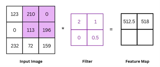
In this example, the size of our image is 3×3 pixels. The size of the filter is 2×2. The size of the filter can vary and is an important hyperparameter, with larger filters potentially capturing more global trends and smaller filters focusing on local details.

Perform convolution between image and filter

To perform the convolution between the input image and the filter, we start from the left corner of the input and then perform element wise multiplication between the filter and the overlapping input image and sum the results for our output.

In simple terms, we are performing the following steps:

(123 x 2) + (210 x 1) + (0 x 0) + (113 x 0.5) = 512.5

We then move to the right by one pixel, and perform the same operation again, as shown below.

Mathematically, we can expand this operation as follows:

(210 x 2) + (0 x 1) + (113 x 0) + (196 x 0.5) = 518

Next, we move the filter to the bottom left of the input image and convolve it with the filter. It is again shifted a pixel to the right to achieve the final feature map depicted below.

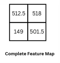
Once we have a complete feature map like above, we pass it through a non-linear activation function, such as ReLU, to introduce non-linearity in the network. Without this essential step, the CNN’s ability to learn complex patterns will be very limited.

Additional Notes

Congratulations! You have made it through the most complicated part of CNNs. Before moving on, there are some additional bits of information to take note of:

1. Convolutional layers typically apply multiple filters in parallel to the input image, generating multiple output feature maps. This is referred to as the ‘depth’ of the layer. Each filter is designed to extract a specific feature from the image: edges, shapes, horizontal lines, texture, etc.
2. For color images with three channels (RGB), each filter is actually a 3-D block, and the convolution includes a sum across all channels. The diagram below illustrates how a filter for an RGB image might look like:

Note that the above diagram only depicts a single filter. The three individual matrices slide over each corresponding color channel of the input image in the same way as before; the sum of the dot product from all three channels is once again summed up to form the feature map.

1. Another important hyperparameter in the convolutional layer is the ‘stride’. In our example above, we have seen how the filter shifts by a pixel across the whole input image to compute the feature map. While this is one way of going about it, it is not the only way. In this context, stride refers to the number of pixels a filter shifts on the input image during the convolution operation. Our initial example had a stride size of 1. The example diagram below illustrates a stride size of 2 with a larger 4×4 pixel image input. The size of the filter remains 2×2.

Just like the size of the filter, the stride size also controls how much granularity and details we want to capture from the image, with a smaller stride size capturing more finer details. However, this could potentially result in model overfitting, which can be mitigated by a larger stride size.

1. Lastly, another hyperparameter in this layer is ‘padding’, whereby we append extra pixels around the edges of the input image manually. Padding can be either uniform (as illustrated below), where we are appending the extra pixels on all the edges of the image equally, or asymmetrical, where padded pixels are placed unequally around the image’s edges.

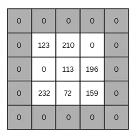
Generally, the zero-padding method is common, as we set the value of padded pixels to zero. The purpose of padding is to ensure that the filter passes over the pixel values in the border region of images multiple times. Without padding, the filter will only pass through some pixels, such as the top right one, only once. Therefore, padding is employed when image borders contain useful information.

Pooling Layer

Once we have acquired our activated feature maps, they typically go through a pooling layer, whose main purpose is dimensionality reduction. Recall that one of the limitations of Neural Networks was scalability when working with image data. Thus, this pooling layer lowers the spatial dimension of data, subsequently lowering the computational resources required, number of parameters, while also introducing partial translation invariance to the model.

The most common pooling method is Max Pooling, where each small patch of the feature map (say 2×2) is reduced to its maximum value. Other methods, such as Mean pooling, also exist, whereby we take the arithmetic mean instead.

Note that in the example above, our window size is 2×2. This is another hyperparameter that can be modified with smaller windows, preserving more spatial resolution, and larger windows, reducing the dimension of the feature map more aggressively. The stride of this window (above example) is also 2 – another knob we can alter to achieve different results.

Lastly, if we work with multiple feature maps, max pooling will be applied independently to each feature map to get the same number of pooled feature maps.

Flattening

CNNs typically stack multiple pairs of convolution and pooling layers. The first few layers might learn to detect edges and colors, the middle layers learn textures and patterns, and the deeper layers begin to recognize parts of objects or entire objects. This hierarchical learning is one of the key strengths of CNNs.

These multiple convolutions and pooling blocks decrease the dimensionality of data but increase the number of feature maps. To feed this data into a standard neural network for the final downstream task, such as classification, we first flatten it into a single vector.

In case of multiple pooled feature maps, as is often the case, we will simply flatten it as it is as well. For instance, if you are left with a 3-D tensor of shape (7, 7, 128) after convolution and pooling layers, it means that you have 128 pooled feature maps of the dimension 7×7. This entire 3-D block is flattened, resulting in a 7 x 7 x 128 = 6272 length long 1-D vector.

This step is undertaken because standard neural networks do not work with multidimensional data. They expect 1D input vectors for which reason flattening is the bridge between the spatial feature representation (in 3D) and the classification layer, where the final prediction is made.

Fully Connected Neural Network

Once we have extracted meaningful features from the image data and reduced its dimensionality, a standard fully connected neural network is the perfect toolkit to translate these features into predictions. Since the readers are likely intimately familiar with neural networks by now, we won’t delve into the technical nitty gritty at this stage. But to sum up, the weighted sum of flattened features is passed through non-linear activation functions across multiple hidden layers of the network before the SoftMax activation function is applied to achieve probability scores for classification purposes.

As is generally the case with machine learning models, this is only half the story. The big question revolves around figuring out the optimal values for model parameters and filter values. Again, as usual, we can find the answer in the backpropagation algorithm for CNNs. Although the technicalities of this algorithm won’t be discussed in this tip, its details can be found in the document: Derivation of Backpropagation in Convolutional Neural Network (CNN).

Implementing a CNN in Python

Now that we have a good foundation to work with, we can begin by implementing our own CNN in Python with the PyTorch framework. For this purpose, we will be working with the CIFAR-10 dataset presented by Krizhevsky et al. The dataset comprises 60,000 32×32 pixel color images in 10 classes, with 6000 images per class. The classes range from images of vehicles to animals.

Import Libraries

To begin, let’s first import the required libraries.

#MSSQLTips.com (Python)
#Importing Required Libraries
import torch
import torch.nn as nn
import torch.optim as optim
import torchvision
import torchvision.transforms as transforms

Load Dataset from PyTorch

Now we can load our dataset directly from PyTorch. Before we can do so, however, it is important to define a transformation that converts the images to PyTorch tensors and normalizes each RGB channel by scaling it between -1 and 1 for a stable and faster training.

#MSSQLTips.com (Python)
#Define Transformations 
transform = transforms.Compose([
    transforms.ToTensor(), 
    transforms.Normalize((0.5, 0.5, 0.5), (0.5, 0.5, 0.5))  
])

Now to load the dataset and apply the said transformation above:

#MSSQLTips.com (Python)
#Loading Dataset
train = torchvision.datasets.CIFAR10(root='./data', train=True, download=True, transform=transform)
trainloader = torch.utils.data.DataLoader(train, batch_size=64, shuffle=True, num_workers=2)
 
test = torchvision.datasets.CIFAR10(root='./data', train=False, download=True, transform=transform)
testloader = torch.utils.data.DataLoader(test, batch_size=100, shuffle=False, num_workers=2)

Note that we are shuffling the data for both train and test splits and then preparing it in batches for memory-efficient model training.

Define architecture of CNN model

Let’s jump to defining the architecture of our CNN model. As an experiment, we will be working with three stacked layers of convolutional and pooling layers. The first convolutional layer of the model accepts three RGB channels as input and outputs 48 feature maps. Hence, 48 filters are being applied in the first layer with a size of 5. Padding is also being employed. The resulting feature maps are then directed through the ReLU activation function before we down-sample each feature map by a factor of 2.

A similar procedure follows for the rest of the stacked convolutional and pooling layers with varying numbers of filters, filter size, and padding. The final feature map has a dimension of (192, 4, 4). The size of these 192 feature maps is 4×4, as we started out with an image size of 32×32 and down-sampled in the max pooling by a factor of 2 layer thrice.

Next, it’s time to flatten this feature map and pass it to a fully connected neural network with a hidden layer containing 384 neurons followed by the output layer for 10 classes.

#MSSQLTips.com (Python)
#Model Definition
class CNN(nn.Module):
    def __init__(self):
        super(CNN, self).__init__()
        self.conv_layers = nn.Sequential(
            nn.Conv2d(3, 48, kernel_size=5, padding=2),  
            nn.ReLU(),
            nn.MaxPool2d(kernel_size=2, stride=2),       
 
            nn.Conv2d(48, 96, kernel_size=3, padding=1),  
            nn.ReLU(),
            nn.MaxPool2d(kernel_size=2, stride=2), 
 
            nn.Conv2d(96, 192, kernel_size=3, padding=1), 
            nn.ReLU(),
            nn.MaxPool2d(kernel_size=2, stride=2)                
        )
 
        self.fc_layers = nn.Sequential(
            nn.Flatten(),                                
            nn.Linear(192 * 4 * 4, 384),
            nn.ReLU(),
            nn.Linear(384, 10)      
        )
 
    def forward(self, x):
        x = self.conv_layers(x)
        x = self.fc_layers(x)
        return x

Initialize CNN model

We now initialize our simple CNN model with its loss function and optimizer.

#MSSQLTips.com (Python)
model = CNN()
loss_function = nn.CrossEntropyLoss()
optimizer = optim.Adam(model.parameters(), lr=0.001)
 
#GPU Use
device = torch.device('cuda' if torch.cuda.is_available() else 'cpu')
model.to(device)

The model’s summary is also shown below:

Specify Training Loop

We can now specify a training loop for our model. Let’s go with 30 epochs and a learning rate of 0.001.

#MSSQLTips.com (Python)
#Model Training
EPOCHS = 30
 
for epoch in range(EPOCHS):
    model.train()
    running_loss = 0.0
    for i, (inputs, labels) in enumerate(trainloader):
        inputs, labels = inputs.to(device), labels.to(device)
 
        # Zero the parameter gradients
        optimizer.zero_grad()
 
        # Forward + backward + optimize
        outputs = model(inputs)
        loss = loss_function(outputs, labels)
        loss.backward()
        optimizer.step()
 
        running_loss += loss.item()
 
    print(f"Epoch {epoch+1} - Training Loss: {running_loss/len(trainloader):.3f}")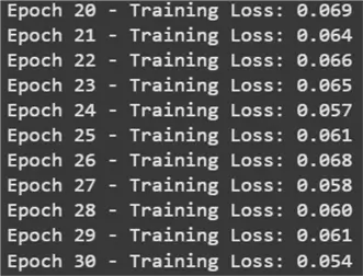

Evaluate the Model

Now, we can evaluate our trained model on the test dataset.

#MSSQLTips.com (Python)
#Model Testing
model.eval()
correct = 0
total = 0
with torch.no_grad():
    for inputs, labels in testloader:
        inputs, labels = inputs.to(device), labels.to(device)
        outputs = model(inputs)
        _, predicted = torch.max(outputs.data, 1)
        total += labels.size(0)
        correct += (predicted == labels).sum().item()
 
print(f"Test Accuracy: {100 * correct / total:.2f}%")

Thus, as you can see, our simple CNN model achieves a decent accuracy of about 74%. If it does not seem like enough, remember that our model specification is still relatively simple, and there are plenty of hyperparameters that can be tuned for more optimal results.

Conclusion

In this tip, we have established basic ideas behind how images are interpreted by modern computers and why traditional neural networks fall short when dealing with visual data. We introduced and explained CNNs – the math and purpose behind each layer of this architecture. To solidify the reader’s understanding of this model, we built our own CNN using PyTorch for the classification of the CIFAR-10 dataset.

Next Steps

• You have multiple tools at your disposal, including data augmentation, hyperparameter tuning, specifying a deeper CNN model with more stacked layers, and so on, to replicate the code above to produce better results.
• Another challenge to explore is to work with the CIFAR-100 dataset, which contains 100 image classes for your model to figure out.
• Interested readers are also advised to check out advanced vision models (ResNet, DenseNet, and EfficientNt) and see how their performance compares to our simple CNN on the CIFAR-10 dataset.
• Moreover, projects involving object detection, semantic segmentation, and instance segmentation should also be investigated as they are key tools in real-world applications like medical imaging, autonomous vehicles, and surveillance.
• Another interesting project to undertake is to build your own image dataset through web scraping. Working with clean public datasets is easy. The real challenge comes in when you must collect your own data, label it, and ensure that there are no biases or class imbalance present. Then employ your custom CNN model or an advanced vision model to solve a real-world problem with this dataset. Lastly, CNNs are not only for images! They surprisingly work quite well for time series data and even for textual data.
• Check out more AI related tips.