Problem
Multivariate analysis in data science is a type of analysis that tackles multiple input/predictor and output/predicted variables. This tip explores the problem of predicting air pollution measured in particulate matter (PM) concentration based on ambient temperature, humidity, and pressure using a Bayesian Model.
Solution
One way to approach multivariate analysis and prediction is to use a Bayesian network model. In Bayesian statistics, we use prior knowledge and information to predict a subsequent result with a certain degree of probability. In this case, we will apply the Bayesian statistical approach to the problem of predicting air quality in micrograms per cubic meter of particulate matter concentration.

For a refresher, please check out the following articles: Bayesian statistics and Bayesian networks. This tip dives directly into a practical approach for implementing these powerful statistical concepts using Python and related packages.
Environment
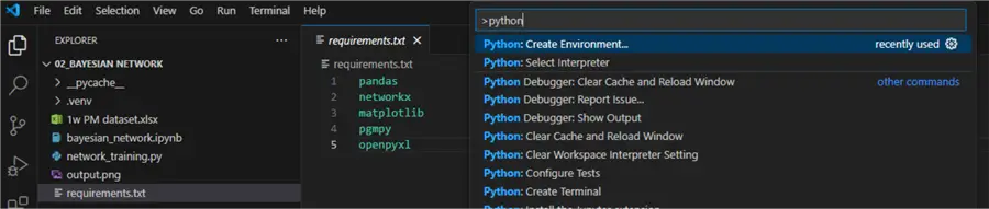
Begin by creating a project folder and opening it in VS Code. Then, create a requirements.txt file containing five lines: pandas, network, matplotlib, pgmpy, openpyxl. Next, press Ctrl+Shift+P and choose Python: Create Environment.
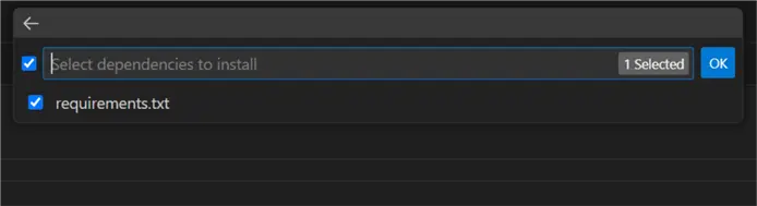
Follow the prompts for creating a local virtual environment. Make sure to check requirements.txt so the environment agent will install the required Python packages directly:
Once you have your environment ready, create an empty .ipynb file in the root project folder. Then proceed to the next steps.
Data Overview
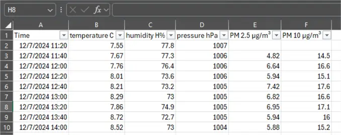
I collected the data for this experiment from a home IoT device. The device continuously collects ambient conditions data:
- Temperature in degrees Celsius
- Humidity in relative percentage
- Pressure in hPa
- Particulate matter concentration of particles up to 2.5 micrometers in diameter in μg/m³
- Particulate matter concentration of particles up to 10 micrometers in diameter in μg/m³
Each set of readings is taken at regular 20-minute intervals, based on the sensor’s setting. Therefore, I decided not to postprocess the data. In case of readings at irregular time intervals, a sampling technique might have been required. The overall data set encompasses a period of one week, from 12/7/2024 until 12/14/2024.
The source file will be provided in case you want to experiment with the data yourself.
Imports and Data Shape
First, let us define the required imports and check the dimensionality of our data:
#MSSQLTips.com (Python)
import numpy as np
import pandas as pd
import networkx as nx
import matplotlib.pyplot as plt
from pgmpy.estimators import BicScore
from pgmpy.models import BayesianNetwork
from pgmpy.estimators import MaximumLikelihoodEstimator
from sklearn.model_selection import train_test_split
data = pd.read_excel(r'1w PM dataset.xlsx',
                     header=0,
                     index_col=None)
print(data.shape)
print(data.isnull().any())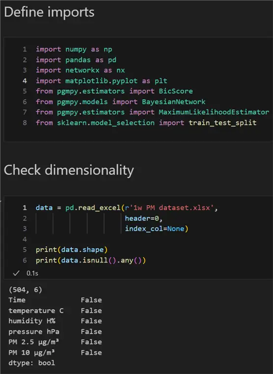
We can see there are 504 rows and 6 columns. There are no null values in the dataset, which is an important prerequisite to continue further.
Discretization
The next order of business for this problem is discretization. Discretization in machine learning refers to converting continuous data to discrete data. Continuous data may take infinitely many values, while discrete data has countable, finite values. For example, the temperature value of 4.5°C is continuous. However, binning the data between 4 and 5 results in a discrete interval (4, 5]. The interval tells us in which range our data falls, in addition to what the lower and upper bounds are. To use the Bayesian modeling approach, we require discrete, or binned, data.
Here is one way to approach the discretization problem:
#MSSQLTips.com (Python)
01: def optimize_bin_width(data: pd.DataFrame,
02:                        column: str) -> float:
03:     """Use Freedman-Diaconis rule for optimal bin width"""
04:     IQR = data[column].quantile(0.75) - data[column].quantile(0.25)
05:     n = len(data)
06:     bin_width = 2 * IQR / (n ** (1/3))
07:     return bin_width
08:
09: def bin_numeric_columns(df: pd.DataFrame,
10:                         numeric_columns: list[str],
11:                         bin_col_mapping=None) -> tuple[pd.DataFrame, dict[str, np.array]]:
12:     discretized_data = df.copy()
13:
14:     if bin_col_mapping is None:
15:         bin_col_mapping = {}
16:         for col in numeric_columns:
17:             bin_width = optimize_bin_width(df, col)
18:             bin_col_mapping[col] = np.arange(
19:                 df[col].min(),
20:                 df[col].max() + bin_width,
21:                 bin_width
22:             )
23:
24:     for col in numeric_columns:
25:         discretized_data[col] = pd.qcut(
26:             discretized_data[col],
27:             q=10,  # or use optimal number of bins
28:             labels=False, duplicates='drop'
29:         )
30:     return discretized_data[numeric_columns], bin_col_mapping
Let’s break it down line by line:
- 01: Define a function to set optimal bin width using an implementation of the Freedman-Diaconis rule.
- 04: Calculate inter-quartile range.
- 05: Get the length of the data set (number of rows).
- 06: Calculate bin width according to the predefined formula

- 09: Define a function to bin columns with parameters the data set (df) and list of numeric columns.
- 15: Create a data structure to store bin to column mapping.
- 16 – 17: For each column, we calculate the appropriate bin width.
- 18: For the current column, store the current range. The range is created using
arange, where the start value is the minimum column value, the end value is the maximum plus thebin_width. The step between values is the bin width. We will use this mapping to store the actual bin edges. - 24: Discretize the data fort each column using decile configuration. This will replace each float value with an index between zero and nine indicating the bin to which each value corresponds.
Here is the result:

Now let us run it:
#MSSQLTips.com (Python)
1: binned_data, bin_col_mapping = bin_numeric_columns(data,
2:                           data.select_dtypes([np.number]).columns)
3:
4: print(binned_data.head())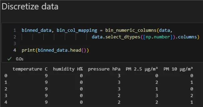
Bayesian Network Structure
Now, we have the data prepared for input to the Bayesian Network. We use the following code to create and visualize the network, displaying how the features influence each other:
#MSSQLTips.com (Python)
01: train_data, test_data = train_test_split(binned_data,
02:                                          test_size=0.2,
03:                                          stratify=None)
04:
05: def plot_network(model, title="Bayesian Network"):
06:     G = nx.DiGraph(model.edges())
07:     pos = nx.spring_layout(G)
08:     plt.figure(figsize=(10, 8))
09:     nx.draw(G, pos, with_labels=True, node_color='lightblue',
10:             node_size=1500, font_size=10, font_weight='bold')
11:     plt.title(title)
12:     plt.show()
13:
14: edges = [
15:     ('temperature C', 'PM 2.5 μg/m³'),
16:     ('temperature C', 'PM 10 μg/m³'),
17:     ('humidity H%', 'PM 2.5 μg/m³'),
18:     ('humidity H%', 'PM 10 μg/m³'),
19:     ('pressure hPa', 'PM 2.5 μg/m³'),
20:     ('pressure hPa', 'PM 10 μg/m³'),
21:     ('PM 2.5 μg/m³', 'PM 10 μg/m³')
22: ]
23:
24: model = BayesianNetwork(edges)
25:
26: plot_network(model, "Initial Bayesian Network Structure")
27: try:
28:     bn_model = BayesianNetwork(model.edges())
29:     bn_model.fit(train_data, estimator=MaximumLikelihoodEstimator)
30:     est = BicScore(test_data)
31:     score = est.score(bn_model)
32: except Exception as e:
33:     print(f"Error fitting the Bayesian Network: {e}")
34:
35: print(bn_model.edges())
36: print(f'Score: {score}')
Let us break it down:
- 01: Define train/test split of the already binned data.
- 05: Define a plotting function.
- 06: Instantiate a direct acyclic graph object to help us plot the network based on the learned edges.
- 09: Draw using typical configuration.
- 11, 12: Add a title, show the plot.
- 14 – 22: Predefine the edge dependency. In a real-world scenario where a lot less may be known about the data or the problem, this step can be skipped to allow the network to provide its own learned dependency mapping between the features. However, as part of this problem, we have assumed that temperature, humidity, and pressure affect the particulate matter concentration. Therefore, we provide a definition for the possible edges.
- 24: Instantiate a Bayesian Network model.
- 26: Plot the network.
- 28: Assign the edges to a variable.
- 29: Fit the training data.
- 30, 31: Estimate a Bayesian Information Criterion (BIC) score. This is a single relative metric that provides an estimation of how good the model is. It is like RMSE in regression problems.
- 35, 36: Finally, print the edges and the score.
Here is the complete code:
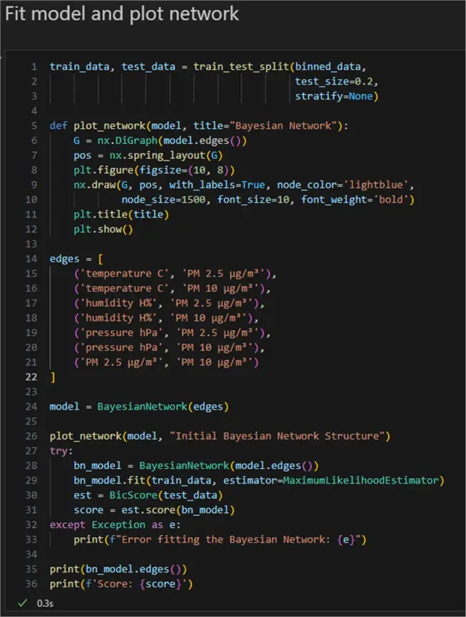
This is what the network looks like:
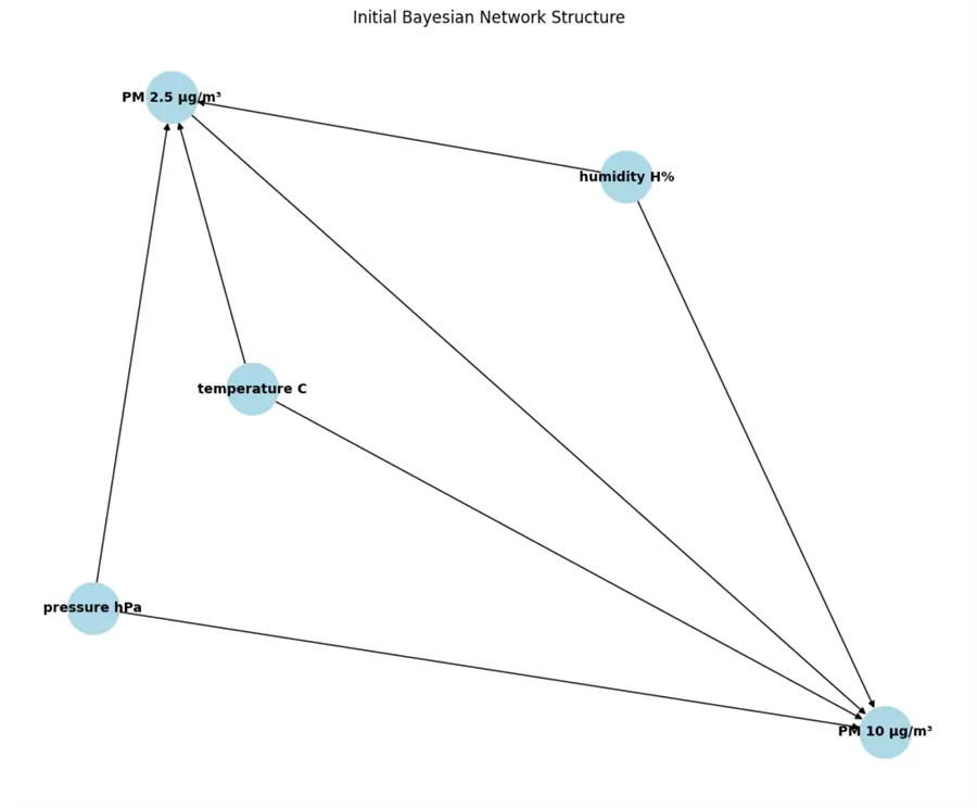
In a scenario with undefined intervariable dependencies, we would see how the network learned the dependencies. Here we see the same result according to our definition. For example, we have the edges going from temperature, humidity, and pressure to PM2.5 and PM10. The Score is the BIC, typically a negative number due to the way it is calculated. The lower the number, the better. Here, I got a score of -206378, the lowest from several experiments I ran previously.

Inference
Our next step is to use the Bayesian network we trained to make a prediction on new data. However, we would not be able to just pass the unseen values of temperature, humidity, and pressure. First, we must see which discrete bins the input values belong to. The prediction we get will also represent a bin number. Therefore, to get a value we can interpret, we must extract range values from the input data based on the predicted bin number:
#MSSQLTips.com (Python)
01: from typing import Any
02: def predict_pm(humidity: float,
03: pressure: int,
04: temperature: float,
05: original_data: pd.DataFrame,
06: bn_model: BayesianNetwork,
07: bin_col_mapping: dict[str, list]) -> dict[str, dict[str, Any]]:
08: try:
09: evidence = {
10: 'humidity H%': pd.cut([humidity], bins=bin_col_mapping['humidity H%'], labels=False)[0],
11: 'pressure hPa': pd.cut([pressure], bins=bin_col_mapping['pressure hPa'], labels=False)[0],
12: 'temperature C': pd.cut([temperature], bins=bin_col_mapping['temperature C'], labels=False)[0]
13: }
14: df_evidence = pd.DataFrame([evidence])
15:
16: pm25_result = bn_model.predict(data=df_evidence, stochastic=False)['PM 2.5 μg/m³']
17: pm10_result = bn_model.predict(data=df_evidence, stochastic=False)['PM 10 μg/m³']
18:
19: pm25_bins = pd.qcut(original_data['PM 2.5 μg/m³'], q=10, retbins=True)[1]
20: pm10_bins = pd.qcut(original_data['PM 10 μg/m³'], q=10, retbins=True)[1]
21:
22: pm25_range = (pm25_bins[int(pm25_result)], pm25_bins[int(pm25_result) + 1])
23: pm10_range = (pm10_bins[int(pm10_result)], pm10_bins[int(pm10_result) + 1])
24:
25: results = {
26: 'PM 2.5': {
27: 'bin': pm25_result,
28: 'range': f"{pm25_range[0]:.1f} - {pm25_range[1]:.1f} μg/m³"
29: },
30: 'PM 10': {
31: 'bin': pm10_result,
32: 'range': f"{pm10_range[0]:.1f} - {pm10_range[1]:.1f} μg/m³"
33: }
34: }
35:
36: print("\nInput values:")
37: print(f"Temperature: {temperature}°C")
38: print(f"Humidity: {humidity}%")
39: print(f"Pressure: {pressure} hPa")
40:
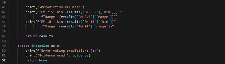
41: print("\nPrediction Results:")
42: print(f"PM 2.5: Bin {results['PM 2.5']['bin']}, "
43: f"Range: {results['PM 2.5']['range']}")
44: print(f"PM 10: Bin {results['PM 10']['bin']}"
45: f"Range: {results['PM 10']['range']}")
46:
47: return results
48:
49: except Exception as e:
50: print(f"Error making prediction: {e}")
51: print("Evidence used:", evidence)
52: return None
- 09 – 14: Define a dictionary containing the “evidence”. These are the predictor (independent) values. The response (dependent) values are all the variables not specified in this dictionary. This is partially where the massive predictive power of a Bayesian network lies – it can learn complex interdependencies between sets of different variables.
- 16, 17: Assign the prediction to variables. The parameter stochastic is important to note. When False, it returns the states with the highest probability value. In the context of this problem, I believe setting it to False is the better choice concerning the amount of data and other settings.
- 19, 20: Bin the independent variables.
- 22, 23: Extract the values from the bins.
- 16, 17: Look up the values of the predicted values according to the discrete predicted bin.
- 25 – 34: Construct result output.
- 36 – 47: Print and return results.
Here is what making a prediction looks like for cold and damp weather:
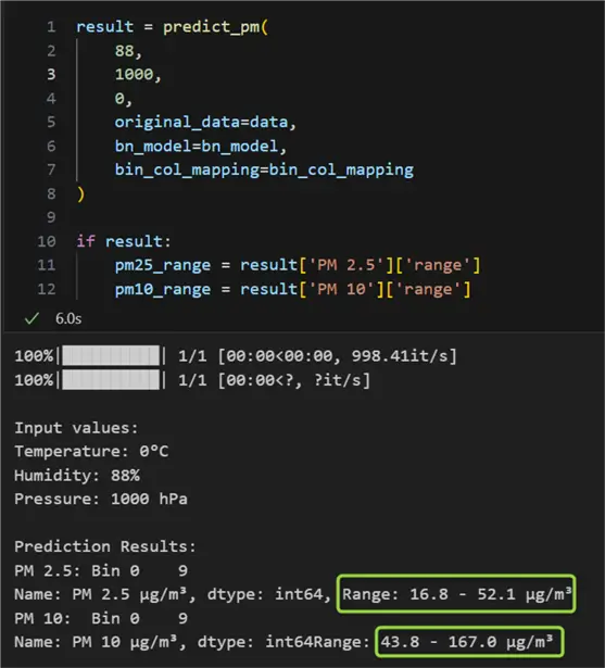
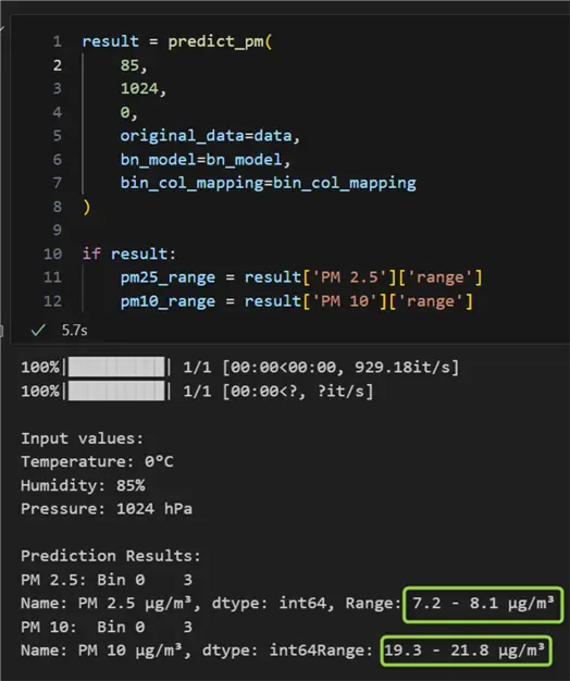
For the provided values of 0°C, 88 %, and 1000 hPa for the independent variables temperature, humidity, and pressure respectively, we received expected ranges of air pollution of 16.8 – 52.1 μg/m³ for PM2.5 and 43.8 – 167 μg/m³ for PM10. According to our model, if humidity decreases, pressure increases, and temperature remains the same, we can expect slightly lower levels of pollution:
Conclusion
This tip has explored setting up a Bayesian network, visualizing it, and using the Bayesian model behind it for predicting air pollution based on other ambient factors such as temperature, humidity, and air pressure. To improve the model, we can consider gathering more data spanning more than one week and more than one season. An additional improvement can be to add a cross-validation model function to pick the best model based on several runs.
Next Steps
