By: Hristo Hristov | Updated: 2023-05-05 | Comments | Related: > Python
Problem
Considering two variables, we want to determine to what extent they are correlated. There are two types of correlation analysis depending on how the two variables relate: linear and non-linear. How do we check if two variables are non-linearly correlated? How do we measure and express their degree of correlation?
Solution
Two variables are non-linearly correlated when their dependence cannot be mapped to a linear function. In a non-linear correlation, one variable increases or decreases with a variable ratio relative to the other. This behavior contrasts with linear dependence, where the correlation between the variables maps to a linear function and is constant. Therefore, in a linear dependence, you see a straight line on the scatter plot, while with a non-linear dependence, the line is curved upwards or downwards or represents another complex shape. Examples of non-linear relationships are exponential, logarithmic, quadratic, or cubic.
Data
Like the last experiment with the linear correlation, we will use a dataset containing machining data but focus on different variables. You can download it here. Here is a preview of the first five out of the total ten thousand rows:

Pair Plots
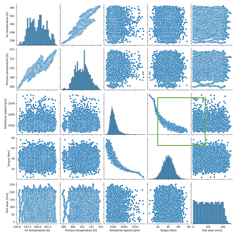
One of the easiest ways to examine visually multivariate data is to generate a pair plot. This type of plot creates a scatter plot for each pair of numeric variables. This is how we can identify a pair that looks non-linearly correlated. A pair plot is easy to generate with the seaborn package. Let's select only the numerical features of interest:
import seaborn as sns

data = data[['Air temperature [K]','Process temperature [K]','Rotational speed [rpm]','Torque [Nm]','Tool wear [min]']]
sns.pairplot(data)

Now let's focus on the relation between Rotational speed in revolutions per minute and torque in Newton meters. The shape of the dot cloud is not a straight line, i.e., the dependency between these two vectors is non-linear for the most part.
Non-linear Correlation
There are many types of non-linear relationships: quadratic, cubic, exponential, or logarithmic. In our example, we can say that as the rotational speed increases, the torque decreases and vice-versa. According to the scatter plot, this relationship appears to be non-linear, i.e., maps to a non-linear function. To calculate the correlation coefficient, we should experiment with methods for calculating non-linear relationships. However, note that our focus here is to express the strength of the relationship rather than to find the closest function that describes the relations. Therefore, doing a regression analysis, which tries to approximate a function close to reality, is out of the scope of this tip.
First, let's define our variables:
x = data['Torque [Nm]']
y = data['Rotational speed [rpm]']
Next, let's examine various methods for calculating the non-linear correlation coefficient.
Distance Correlation
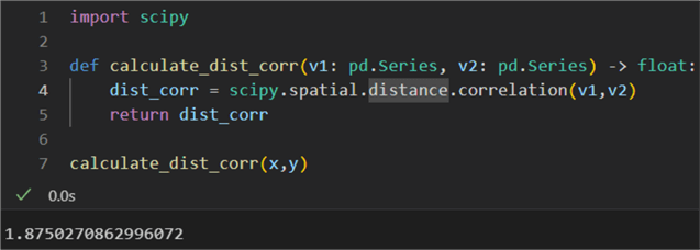
This metric can be applied to both linear and non-linear data. Its advantages are that it does not assume the normality of the input vectors, and the presence of outliers has a reduced influence on it. The results range from 0 to 2, where 0 means perfect correlation and 2 means perfect negative correlation.
1: import scipy
2:
3: def calculate_dist_corr(v1: pd.Series, v2: pd.Series) -> float:
4:     dist_corr = scipy.spatial.distance.correlation(v1,v2)
5:     return dist_corr
6:
7: calculate_dist_corr(x,y)
The result is 1.85, so as expected, there is a strong reverse dependence between torque and rotational speed:

Mutual Information
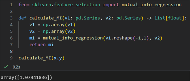
Mutual information (MI) between two random variables is a non-negative value ranging from 0 to +∞. Results around 0 mean the variables are independent. On the other hand, the higher the value, the more interdependent the two variables are. MI is called this because it quantifies the information the two variables share. However, results can be difficult to interpret because there is no higher bound to the max MI possible. For example:
1: from sklearn.feature_selection import mutual_info_regression
2:
3: def calculate_MI(v1: pd.Series, v2: pd.Series) -> list[float]:
4:     v1 = np.array(v1)
5:     v2 = np.array(v2)
6:     mi = mutual_info_regression(v1.reshape(-1,1), v2)
7:     return mi
8:
9: calculate_MI(x,y)
Let's break it down:
- To calculate MI, we need the scikit learn package, so we import it on line 1.
- On line 3, we define a function accepting two vectors and returning a list of floats, the MI coefficient for each pair (here just one pair)
- On lines 4 and 5, we convert the pd.Series objects to numpy arrays.
- Finally, on line 6, we calculate MI.
The result is:

Again, we get a strong correlation, considering the higher bound is non-existent.
Kendall's Tau
Kendall rank correlation coefficient, or Kendall's τ coefficient, is a statistic used to measure the dependence between two ordinal values. Kendall's tau is a useful measure of dependence in cases where the data is not normally distributed or where outliers may be present. While our variables are not ordinal, we can still use Kendall's coefficient like we used Spearman's to measure linear dependence. The coefficient ranges from -1 to 1.
1: def calculate_Kendall(v1: pd.Series, v2: pd.Series) -> tuple[float]:
2:     tau, p_value = scipy.stats.kendalltau(v1, v2)
3:     return tau, p_value
4:
5: calculate_Kendall(x,y)

The result is -0.75, meaning a strong negative correlation. The probability value
(p_value) of 0 indicates we can reject the null hypothesis
of an absence of association (where tau would be 0).
Maximal Information Coefficient
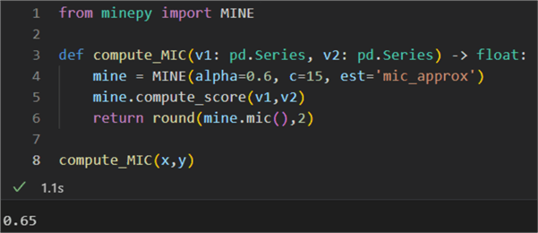
Finally, we can also calculate the maximal information coefficient (MIC). As we have shown previously, this robust correlation measure applies equally well to both linearly and non-linearly correlated data. The coefficient ranges between 0 and 1. Therefore, it is not helpful in showing the direction of the dependence.
1: from minepy import MINE
2:
3: def compute_MIC(v1: pd.Series, v2: pd.Series) -> float:
4:     mine = MINE(alpha=0.6, c=15, est='mic_approx')
5:     mine.compute_score(v1,v2)
6:     return round(mine.mic(),2)
7:
8: compute_MIC(x,y)

Conclusion
This article examined four methods for calculating the correlation coefficient between non-linearly correlated vectors: distance correlation, mutual information, Kendall's tau, and Mutual Information Coefficient. Each has different bounds and captures the relationship between the variables differently. Therefore, using more than one to corroborate or reject a certain theory is standard practice.
Next Steps
About the author
 Hristo Hristov is a Data Scientist and Power Platform engineer with more than 12 years of experience. Between 2009 and 2016 he was a web engineering consultant working on projects for local and international clients. Since 2017, he has been working for Atlas Copco Airpower in Flanders, Belgium where he has tackled successfully multiple end-to-end digital transformation challenges. His focus is delivering advanced solutions in the analytics domain with predominantly Azure cloud technologies and Python. Hristo's real passion is predictive analytics and statistical analysis. He holds a masters degree in Data Science and multiple Microsoft certifications covering SQL Server, Power BI, Azure Data Factory and related technologies.
This author pledges the content of this article is based on professional experience and not AI generated.
View all my tips
Article Last Updated: 2023-05-05


