Problem
Time does surely fly. I remember when Databricks was released to general availability in Azure in March 2018. This means data engineers have been developing Azure Databricks Spark programs for seven years. Many technological changes have been made over that time. Understanding the different ways to process files is key since many different techniques might be used in your environment. How can we get familiar with Azure Databricks with Spark Dataframes?
Solution
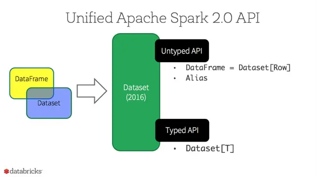
The image below shows that this dataset technology was available in Spark 2.0 around 2016. What is the key difference between a dataframe and a dataset? It is the underlying language. If you are writing code in Python, you are using a DataFrame, which is loosely typed. On the other hand, the Scala language is based on object-oriented Java. Thus, the Spark technology is called a Dataset, which is strictly typed. To learn more about the technology during this time period, please read this article by the engineering team at Databricks.
Business Problem
Our manager has asked us to investigate how to load files into our Delta Lakehouse. This main project will review the different ways to accomplish this task. Today’s proof of concept focuses on PySpark DataFrames and uses delimited data files from the AdventureWorks database. These files are in pipe-delimited format and do not have any headers. Please see this Microsoft Learn link for details. To be successful, the following topics will be reviewed and mastered.
| Task Id | Description |
|---|---|
| 1 | POC Overview |
| 2 | Creating Spark Clusters |
| 3 | Managing Storage |
| 4 | Full Load Pattern |
| 5 | Examine Hive Tables |
| 6 | Simple Workflow |
| 7 | Complex Workflow |
| 8 | Incremental Load Pattern |
At the end of this article, the data engineer will have a working knowledge of the DataFrames and will be able to schedule those pipelines with workflows.
POC Overview
Many older installations of Azure Databricks do not have Unity Catalog enabled. During today’s investigation, I will point out features that are only available in Unity Catalog. The first two notebooks mount the Azure Data Lake Storage to our workspace and clean up our test environment. The full load pattern notebook is good for small to medium size files. The incremental load pattern notebook starts with a full load. Depending on the total size, this might be an iterative approach. Then new files that contain changes are MERGE INTO the final Delta Table. Before workflows, a developer could schedule just a single notebook. We will explore how to call other notebooks using the dbutils library. The ability to add dependencies, monitoring, and alerting is why workflows are awesome.
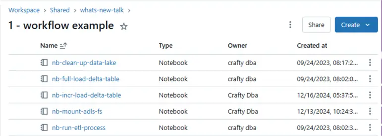
The above image shows the notebooks that we will be exploring. I will include all the code at the end of the article bundled into a zip file format.
Creating Spark Clusters
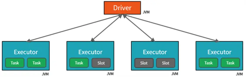
There are several options when creating a computing cluster. Each cluster has one driver and multiple executors. Each slot represents a virtual central processing unit (CPU). The notebook code is converted to Java byte code. A given task can be executed in a single slot and can consume one partition of data. Thus, a Spark job that works with a file that has 10 partitions will require two stages. The first stage will process eight partitions, while the second will consume the last two processes.
All-Purpose Compute Cluster
First, an interactive or “All-purpose compute” cluster is used for data engineering. Set the terminate after n minutes limit configuration so that computing resources are not wasted. The “Job compute” cluster is used when a workflow is started. It automatically terminates at the end of the workflow. The “SQL warehouses” computing is defined using t-shirt sizes and can be used for interactive queries against the local “hive_metastore.”

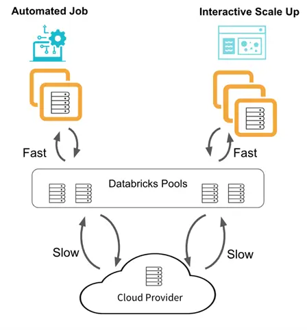
The problem with the first two types of computing is the time for the cluster to deploy and configure infrastructure. This can take 4 to 7 minutes. Pools can reduce this time by increasing the time in which nodes (virtual machines) live. Thus, if we have a pool termination limit of 60 minutes and a cluster termination limit of 15 minutes, we will have nodes staying warm for one hour. This reduces the start time for future calls drastically. However, we still need to deploy the nodes the first time they are used from the pool. See the image below for details.
Setting Cluster Properties
Many properties can be set on a cluster. I am creating a three-node fixed-size cluster that uses a “no isolation shared” access method. Please see the image below that shows the cluster named clsMsSqlTips.
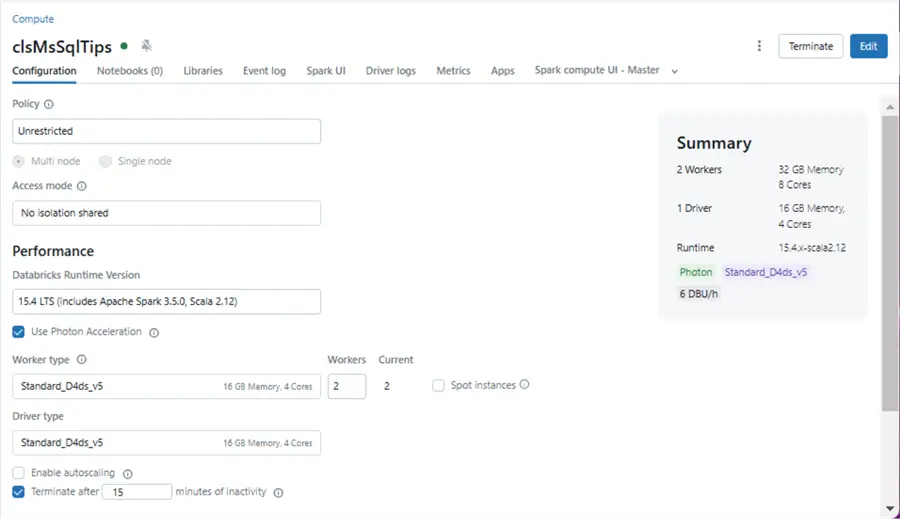
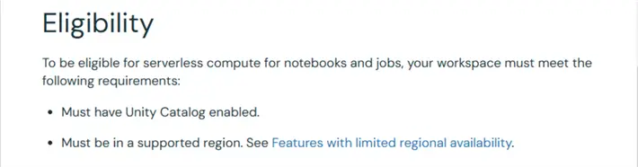
By not having Unity Catalog, we are missing a new feature. Serverless compute is always warm since it comes from a pool of virtual machines owned by Databricks. Therefore, no resources are deployed to our Azure Subscription.
Numerous security concepts have been replaced with Unity Catalog. Credential passthrough was used to place the security management on the Azure Data Lake Storage layer. The identity of the user’s Entra Id is used to enforce both RBAC and ACL rules. When table access controls are enabled on the cluster, the developer can only use Python and SQL to manage the Delta Lakehouse. The GRANT, REVOKE, and DENY statements can be executed from Spark SQL to apply permissions to the tables. I will do an in-depth article on security within Unity Catalog in the future.
Managing Storage
The image below shows a notebook named “nb-mount-adls-fs” that takes the storage account name, the storage container name, and the mount point as input. This depends on a Databricks Secret Scope that is backed by Azure Key Vault. Within this key vault is the tenant id, client id, and client password. This service principle is leveraged when users connect to the mounted storage. Make sure you give both RBAC and ACL access to the service principle.

The next notebook drops any existing tables from the dim and fact schemas. We can also view the contents of the Azure Data Lake Storage by using the list (ls) command in the file system (fs) class from the dbutils library.

We can see the second version of the AdventureWorks folder has a bronze quality layer. Within that layer are two directories named dim and fact.
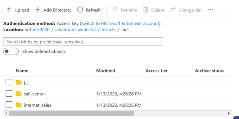
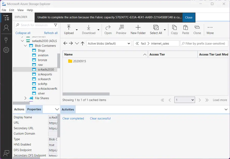
Today, we assume that external processing drops files into the bronze quality zone. The image above is from the Azure Portal storage browser. The fact schema (parent folder) has two tables (child folders). Inside each folder is a delimited file containing the table data.

The above image shows the internet sales table (child folder) in the fact schema (parent folder). There is a logical mapping of the database, schema, and table to the storage locations in the Azure Data Lake. It helps users easily identify the data located in the source system. Of course, a CSV file is not a SQL Server table.

The main purpose of the “nb-clean-up-data-lake” notebook is to clear out the silver storage area and drop hive silver tables. The above image shows two empty schemas.
Full Load Pattern
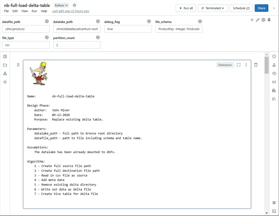
The header for the “nb-full-load-delta-table” notebook is shown below. The following parameters can be passed to the program:
- Data file path (path of the source files)
- Data lake path (static mount point)
- Debug flag (print out details)
- File schema (a string representing the table in DDL format)
- File type (the format of the file)
- Partition count (how many files to write)
Review Notebook Code
Let us take a close look at all the code within the notebook. The code below shows the widgets class within the dbutils library. A widget is just another name for a parameter. The removeAll method drops all existing widgets.
#
# Run one time
#

# dbutils.widgets.removeAll()
Python Code to Define Widgets
The Python code below defines the widgets using the text method. If the widgets do not exist, they are defined. If they exist, the code performs no operation.
#
# Input parameters for notebook
#

# define the lake path
dbutils.widgets.text("datalake_path", "/mnt/datalake/adventure-works-v2/bronze/")

# define the file path
dbutils.widgets.text("datafile_path", "/dim/product/")

# define the debugging flag
dbutils.widgets.text("debug_flag", "true")

# define file type
dbutils.widgets.text("file_type", "csv")

# define partition count
dbutils.widgets.text("partition_count", "2")

# define schema ddl
dbutils.widgets.text("file_schema", "ProductKey  integer, ProductAlternateKey  string, ProductSubcategoryKey  integer, WeightUnitMeasureCode  string, SizeUnitMeasureCode  string, EnglishProductName  string, StandardCost  decimal(19,4), FinishedGoodsFlag  boolean, Color  string, SafetyStockLevel  integer, ReorderPoint  integer, ListPrice  decimal(19,4), Size  string, SizeRange  string, Weight  double, DaysToManufacture  integer, ProductLine  string, DealerPrice  decimal(19,4), Class  string, Style  string, ModelName  string, EnglishDescription  string, StartDate  timestamp, EndDate  timestamp, Status  string")
The get method of the widget class returns the current value. The code below creates a full path to the source directory by combing two parameters. The data file path will be changed for each source folder (table).
#
# 1 - Get full src path to file
#

# remove slash from dir path
full_src_path = dbutils.widgets.get("datalake_path")[:-1] + dbutils.widgets.get("datafile_path")

# debugging
if (dbutils.widgets.get("debug_flag") == 'true'):
  print("1 - create source file path")
  print(full_src_path)
The image below shows the resulting source file path.

Code with source and destination path
Unfortunately, Python creates a shallow copy of a string array. Thus, if we want both the original source path and the new destination path, we need to have two variables. The source path contains parts that translate to the hive schema and hive table. The destination path has all delta tables in the same directory. The code below creates the destination path.
#
# 2 - Make full dst path to file
#

# split into parts
path_parts = full_src_path.split("/")
temp_parts = full_src_path.split("/")

# replace quality zone
temp_parts[4] = 'silver'

# make file name
file_parts = temp_parts[5] + "." + temp_parts[6] + ".delta"
del temp_parts[-1]
del temp_parts[-1]
temp_parts[5] = file_parts

# final file (dir) name
full_dst_path = '/'.join(temp_parts)

# debugging
if (dbutils.widgets.get("debug_flag") == 'true'):
  print("2 - create destination file path")
  print(full_dst_path)
The image below shows the resulting destination file path.

Code to Consume All Files in Each Sub-directory
The code below used the read method of the Spark library to consume all files in each sub-directory. If there are only files in the root directory, it will pick those up too.
#
# 3 - Read csv file
#

# include library
from pyspark.sql.functions import *

# get widget values
partition_count = int(dbutils.widgets.get("partition_count"))
file_schema = dbutils.widgets.get("file_schema")
file_type = dbutils.widgets.get("file_type")

# read in the csv file
df = (spark.read
  .format(file_type)
  .option("header", "false")
  .option("delimiter", "|")
  .option("quote", "")
  .option("recursiveFileLookup", "true")
  .schema(file_schema)
  .load(full_src_path)
)

# debugging
if (dbutils.widgets.get("debug_flag") == 'true'):
  print("3 - read in csv file")
  display(df.limit(5))
The image below shows that the CSV source file(s) have been loaded into a dataframe. If you click the dataframe (df) link, you can view the schema definition. This matches what was passed in as a parameter.

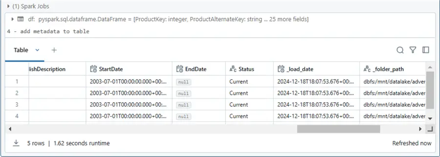
The dataframe withColumn method allows the developer to create new fields. The code below adds the _load_date and _folder_path to the final dataframe.
#
#  4 - Add metadata
#

# add load date
df = df.withColumn("_load_date", current_timestamp())

# add folder date
df = df.withColumn("_folder_path", input_file_name())

# debugging
if (dbutils.widgets.get("debug_flag") == 'true'):
  print("4 - add metadata to table")
  display(df.limit(5))
If we saved the dataframe without adding metadata, we would have no idea what sub-directory a file might be coming from. The idea of packing data into folders named as a sortable string is key to incremental loading without using check points. See the current_timestamp and input_file_name Spark function for details.
The code below uses the remove (rm) method of the file system (fs) class in the dbutils library to remove the existing delta file directory. The repartition method enforces the number files and the write method saves the dataframe as a delta table.
#
# 5/6 - Write delta file
#

# Remove directory via os
try:
  dbutils.fs.rm(full_dst_path, recurse=True)
except Exception:
  pass

# Write out delta table
df.repartition(partition_count).write.format("delta") \
  .mode("overwrite") \
  .save(full_dst_path)

# debugging
if (dbutils.widgets.get("debug_flag") == 'true'):
  print("5 - remove destination folder")
  print("6 - write delta file folder")
The output from executing this cell is just two descriptive messages if debugging is turned on.

The code below uses Spark SQL to DROP TABLE and CREATE TABLE statements.
#
# 7 - Create table using delta file
#

# Make spark sql stmt
sql_stmt = """
  DROP TABLE IF EXISTS {}.{}
""".format(path_parts[5], path_parts[6])

# Remove table
try:
  spark.sql(sql_stmt)
except Exception:
  pass

# Make spark sql stmt
sql_stmt = """
  CREATE TABLE IF NOT EXISTS {}.{}
  USING DELTA
  LOCATION '{}'
""".format(path_parts[5], path_parts[6], full_dst_path)

# Create table
spark.sql(sql_stmt)

# debugging
if (dbutils.widgets.get("debug_flag") == 'true'):
  print("7 - create hive table based on delta file")
  print(sql_stmt)
The output below shows the successful creation of a hive table over the delta file that is stored in Azure Data Lake Storage.

Examine Hive Tables
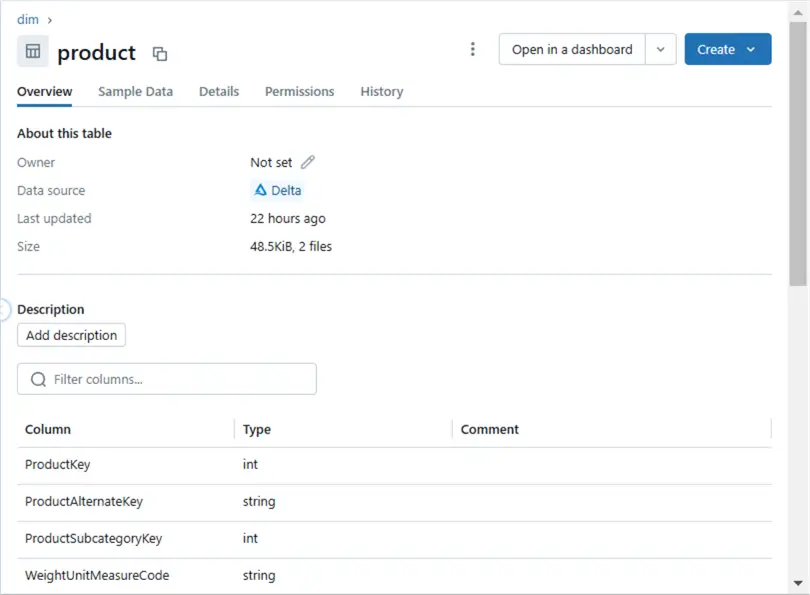
Since we manually executed the full load notebook with parameters for the product source table, we can view the results via the Catalog Explorer. The History section of the table dialog box shows the different actions executed on the delta table. The first action is a WRITE table.

The Overview section of the table dialog box shows key information such as owner, file type, file date, and file size.
The Sample Data section of the table dialog box shows up to the first 1000 rows.

The Details section of the table dialog box displays the table type and table location. We can see that the product table is unmanaged (external).

Finally, we need to have table access controls enabled on the cluster to see table permissions. This is a requirement for workspaces since we do not have Unity Catalog enabled.

The dialog boxes are just a nice interface to existing Spark functions. Please see this article on the statements that can be used to retrieve this data from a Spark query.
Now that we have a product to fully load the AdventureWorks database, how can we schedule a job to rebuild the schema on a recurring basis?
Simple Workflow
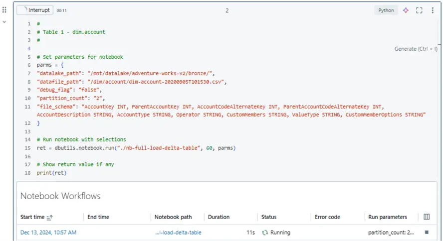
The “nb-run-etl-process” notebook uses the run method of the notebook class in the dbutils library. The screenshot below shows a dictionary called parms thatcontains the parameters we are passing to the full load notebook. These are the same widgets that we can manually update by hand to have the program load different source files into delta tables.
We can create a new workflow called “job-01-before-workflows”. Two key items that the developer must supply are the path to the notebook to run and the Spark cluster. Since this master notebook calls the full load notebook with the parameters for each table, there are no parameters that need to be supplied. The main advancements on this page are the job notifications and duration settings. Please see article 1 and article 2 from the Databricks technical blog for more details. Please note that the computing power for this job is based on an interactive cluster named clsMsSqlTips.

After successful completion of the job, we can use the Catalog Explorer to see all the tables in the two schemas. The details can be found in the image below.

The previous method of creating a parent notebook and calling child notebooks did not have the same level of control as workflows. For instance, who do we notify upon start, failure, completion, or duration? Additionally, adding dependencies in the notebook introduced a bunch of additional code. In the next section, we will see how workflows allow the developer to easily enforce dependencies.
Complex Workflow
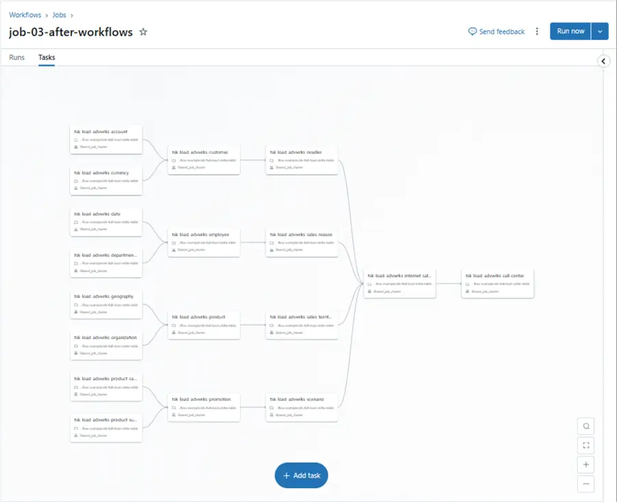
There is nothing new here. Instead of embedding the notebook executions in a parent notebook, we add the calls and parameters to the workflow. Task dependencies are created by referencing prior tasks that need to be completed before executing the current task. Databricks added enhanced control flow mechanisms to workflows in November 2023. The new conditional task type allows for checking on a condition and branching accordingly. Please see this article for details. The image below has the details for the account dataset.

The image below shows an example of a complex workflow. The reseller load process depends on the customer load process being completed successfully. The customer load process depends on both the account and currency loads being completed.
Unlike the parent notebook design, the complex workflow captures the execution timeline. This detail is shown below. We can see that a significant amount of time (5 minutes) was spent spinning up the cluster. The rest of the workflow tasks took less than 30 seconds to execute per call. Please note that the workflow is using a job cluster.

Briefly, workflows supply the developer with more control over dependencies, many ways to alert on tasks, and an effortless way to monitor/visualize runtime executions.
Incremental Load Pattern
Every incremental pattern starts with a full load. Then, on a given schedule, new data files are dropped into the data lake. These files represent changes to the source datasets.
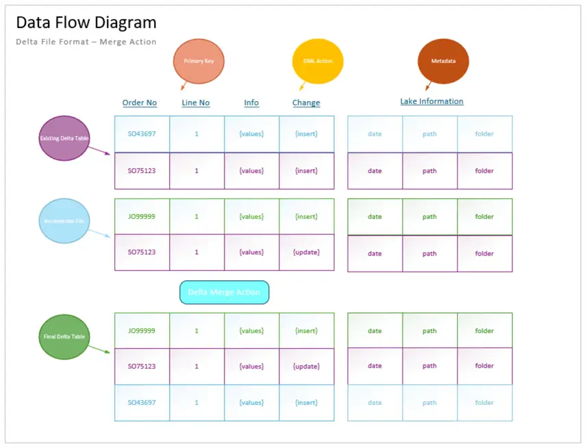
Let us look at a simple diagram I created for the fact internet sales table. Every data file that is sent over must have a primary key. We use this key when merging the existing delta table with the new incremental file (Spark dataframe). Optionally, we need to know the data manipulation action. Does the new record in the file represent an insert, update, or delete? If we do not have this information, we can only support insert and update actions. Adding metadata about the file location is important since the sortable date sub-folder can be used to find the most recent record. The whole incremental pattern is dependent upon the Spark MERGE INTO statement. To be more specific, I like the dataframe method so that I do not need to list all the fields in the delta table.
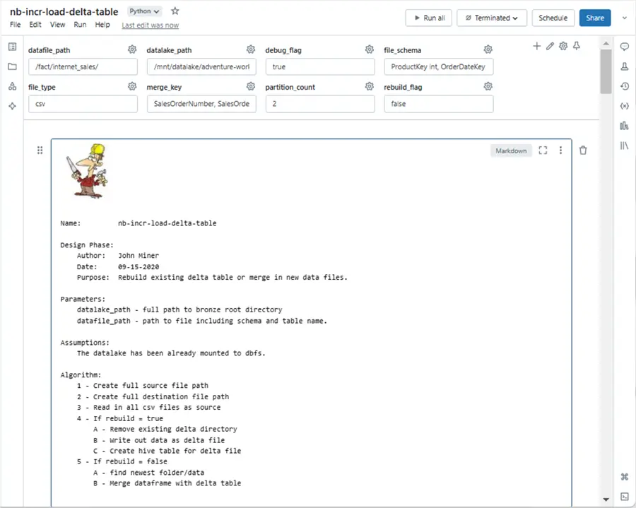
Review What is Different Between Notebooks
I will only cover what is different between the notebooks. It is especially important to document the algorithm of a complex notebook. We can see that the merge key (primary key) is how we will join the two tables. The rebuild flag is when we must rebuild the table from the existing files.
Unlike before, the data files must reside in a date-stamped folder. The image below shows Azure Storage Explorer being used to manage files and folders.
Please note that after execution, two new metadata fields are added by the notebook to the dataframe. The folder date and file name are parsed out of the full folder path by the Python code.

Because we are doing more complex processing, we want to get record counts from the delta table before and after a notebook cell execution. The code for a rebuild is the same as a reload.

To test the merge code, we need to create a sample file. The image below shows the SO75123 and JO99999 orders. The first record is an update, and the second record is an insert. Please ignore the dates since this is historical data.

Again, the process of dropping new files into date stamp folders is not the responsibility of the Databricks program. In this case, we are manually doing those tasks.

Code to Retrieve Record Counts from Delta Table
A large part of the code below is used to retrieve record counts from the delta table before the merge, the incremental dataframe, and the delta table after the merge. The for Path method of the Delta Table library allows the developer to interact with a table. Please see the tutorial on upserting data using a Delta Table.
#
# 5 - Rebuild delta table (FALSE)
#

if (rebuild_flag != 'true'):

  # show counts before processing
  try:
    stmt = f"select count(*) as total from {silver_table}"
    cnt = spark.sql(stmt).collect()[0][0]
    print(f"before processing - (table : {silver_table}) - (rows = {cnt})")
  except:
    cnt = 0
    print(f"before processing - (empty table : {silver_table}) - (rows = {cnt})")
  print("")

  # max date
  max_date = df.select(max('_folder_date').alias('max_date')).collect()[0][0]

  # just recent data
  df = df.filter(col("_folder_date") == lit(max_date))

  # show new file counts
  try:
    cnt = df.count()
    print(f"before processing - (dataframe) - (rows = {cnt})")
  except:
    cnt = 0
    print(f"before processing - (empty dataframe) - (rows = {cnt})")
  print("")

  # merge info exists, create condition
  if merge_key:
    merge_keys = merge_key.replace(' ', '').split(",")
    condition = ""
    for keys in merge_keys:
      condition = condition + "existing.{} = updates.{} and ".format(keys, keys)
    if len(condition) > 4:
      condition = condition[:-5]
    print(f"merge condition - {condition}\n")

  # read existing table
  delta_table = DeltaTable.forPath(spark, full_dst_path)

  # merge updates
  delta_table.alias("existing") \
    .merge(source=df.alias("updates"),condition=f"{condition}") \
    .whenMatchedUpdateAll().whenNotMatchedInsertAll().execute()

  # debugging
  print(f"read data from {full_src_path}{max_date} and apply changes to {silver_table} at \n {full_dst_path}\n")

  # show counts after processing
  try:
    stmt = f"select count(*) as total from {silver_table}"
    cnt = spark.sql(stmt).collect()[0][0]
    print(f"after processing - (table : {silver_table}) - (rows = {cnt})")
  except:
    cnt = 0
    print(f"after processing - (empty table : {silver_table}) - (rows = {cnt})")
  print("")
Output from Executing Python Code
The image below shows the output from executing the above Python code. We can see two new records are in the incremental file. One was inserted into the table, and one was updated.

It is particularly important to create test cases for your code. If we look for new order dates, we can see the two new records. Please note that you may want to use the SQL Warehouse for queries since the serverless computing is quick.

Does this code work for every use case? The answer is no. First, the rebuild action recursively reads in all files. If we are doing mock deletes, then we are only inserting data during a rebuild. We must add a filter that ranks the order of each record by primary key and folder date descending. Picking the topmost record with row number of one will result in the correct state for the Delta Table. For extremely large files and/or requirements that must delete records, we need to process the files in order. Thus, we need to split the incremental file into two. Records that require a delete and records that are inserts or updates. New Python code for deleting records needs to be added by the developer to the existing notebook.
To recap, incremental loads are especially important when we are dealing with large datasets. Typically, these datasets are partitioned by a hash key such as the year and month of the order date. This partition helps when query patterns typically need a subset of the whole.
Summary
The Azure Databricks service has been around for at least half a decade. This means there are many notebooks in production. During that time, the ways data can be ingested have changed. Today, we talked about using the traditional read and write features of Spark. The Delta File format add ACID properties to Hive Tables. This should be the default format that you save data in the medallion architecture.
Every data engineering notebook that loads data can be classified as either FULL or INCREMENTAL. Additional notebooks that clean, aggregate, or de-normalize data can be used in the gold or platinum layers. Today, we worked with the AdventureWorks data files that were stored in a delimited format.
Scheduling notebooks and enforcing dependencies was harder in the old days with simple jobs. The master notebook had to use code to enforce these rules. Databricks added workflows so that developers could move that code into a graphical user interface that did all the work for them. Workflows give the developer more control over dependencies, many different ways to alert on tasks, and an effortless way to monitor/visualize runtime executions.
Next time, we will talk about autoloader, which uses structured streaming and checkpoints to find new files and ingest them into our Delta Tables. As previously mentioned, here is a zip file with all the notebooks that were reviewed today. Additionally, the delimited files for AdventureWorks are included in the bundle.
Next Steps
- Advanced Data Engineering with Databricks
- What is the Databricks Community Edition?
- Various Databricks Certifications
- Solving problems with Graphframes
- Introduction to ML Flow within Databricks
- Data Governance with Databricks Unity Catalog
- Check out these other Azure Databricks articles
