By: Siddharth Mehta
Overview
The mining structure editor contains five views: Mining Structure, Mining Models, Mining Model Viewer, Mining Accuracy Chart, and Mining Model Prediction. In this chapter we will cover the Mining Structure, Mining Models and the Mining Model Viewer that relates to the configuration and analysis of the data mining model.
Explanation
By default, once you complete the creation of the mining structure, you will be taken to the mining structure view. Follow the below steps to configure and analyze the data mining model.
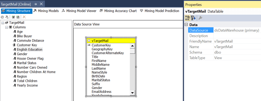
1) The mining structure view contains two panes - the Data Source View (DSV) pane that shows the tables used by the mining structure and the pane on the left that shows the columns of the mining structure in a tree view. You can add / remove columns to the mining structure by dragging and dropping them from the DSV. The properties of a column can be edited in the properties pane when the column is selected.
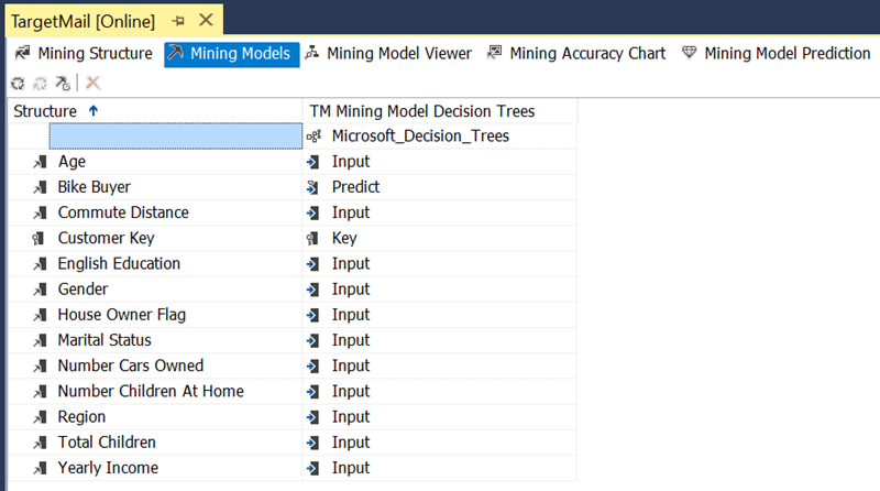
2) The Mining Models view shows the mining models in the current mining structure. You can have one or more mining models within each mining structure. The mining structure editor is used to make refinements to the mining model created by the Data Mining Wizard. Each column of a mining structure can be used for a specific purpose in a mining model - Input, Predict Only, Predict, and Ignore. These usages can be selected from the drop-down list box corresponding to a column in a mining model.
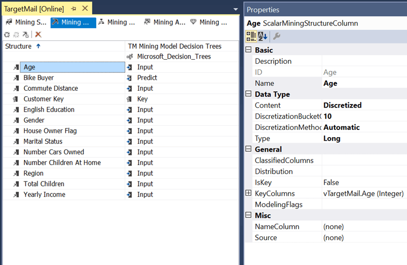
3) Change the usage of the Bike Buyer field to "Predict" as our intention is to predict whether a particular customer would potentially buy bikes. Also, change the Content property to "Discretized" and the DiscretizationBucketCount property to "10", as we do not want to see individual ages, instead we want to see ranges of ages.
4) Press F5 to deploy the data mining model. Once deployment completes, you will be taken to the Mining Model Viewer.
- The decision trees algorithm identifies the attributes influencing customers to buy bikes and splits customers based on those attributes.
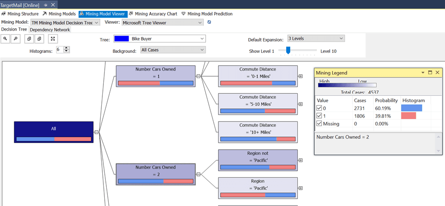
- In the tree view that represents the mining model, the root of the tree starts with a single node that represents all the customers. Each node shows the percentage of customers who have bought bikes based on the input set.
- In the Mining Model Viewer, you can select the depth / level of the tree to view using the Show Level slider. The Mining Legend window shows the legend for the colors in the horizontal bars of a node. Blue indicates customers who are not bike buyers and Red indicates the customers who have bought bikes, and white indicates customers for whom the Bike Buyer value is missing.
- As per this model, the most important attribute that determines a customer buying a bike is the number of cars owned by the customer. If you click the node with "Number Cars Owned = 2", you can see that "39.47%" of such customers are likely to be bike buyers as shown below.
- In this way, you can navigate the tree from each node to identify the attributes that affect a customer's decision to buy a bike.
This completes the development of the data mining model. In the next chapter we will look at testing and validation of this model.
Additional Information
- Consider analyzing the source dataset as well as the model developed by the algorithm in detail to understand how accurately it reflects the structure of the data.
- Click on the Dependency Network tab to analyze the model using a different visualization.
- Click on the viewer drop-down to select an alternate view - Microsoft Generic Content Tree Viewer to analyze the model content in detail.