Logistic Regression and K-Fold Cross Validation in Machine Learning

Problem

As we dive deeper into machine learning (ML), we can focus on another important classifier—Logistic Regression. This model is often the go-to model for binary classification problems. While its name includes “regression,” Logistic Regression serves as a classification algorithm, making it crucial to learn how it operates and differs from linear regression. In this tip, we will introduce this model, alongside another essential technique called K-Fold cross-validation, which will help us locate the better hyperparameters for our model.

Solution

In previous tips, we explored classification algorithms with the K-Nearest Neighbor (KNN) and the Naive Bayes classifier, both simple yet powerful ML models that allow for binary and multi-class classifications. We then also explored how the Linear Regression model works. By now, our journey through these models has likely put you at ease with the general nomenclature used by ML scientists, what problems to expect, and what nitpicky details to look out for. Therefore, to advance this journey into the intermediate stage, this tip will explore the Logistic Regression classifier, an important stepping stone for understanding Neural Networks.

Logistic Regression Introduction

Logistic Regression is a widely used algorithm in real-world applications due to its simplicity, interpretability, and effectiveness for binary classification problems. In the medical domain, it can be employed for automating the diagnosis of low-risk diseases, like predicting if a person has tooth cavities. In the financial and banking sectors, it can be employed for fraud detection based on historical transaction data. Most interestingly perhaps, this classifier can also be used by epidemiologists to model the spread of a disease and see which individual will contract a disease based on their interactions, social behaviors, and demographics. In short, this versatile tool is useful in a variety of fields.

Logistic Regression Basics and Decision Making

Logistic Regression is a supervised learning classification method. It is a linear discriminative parameter model which in short means that the model learns a finite set of parameters to form a linear decision boundary that best separates different classes in the dataset. Fundamentally, this model is primarily designed for binary classification, but with a few tweaks as we will see later, perform multiclass classification as well. The model works by estimating the probability that a particular data point belongs to a certain class. If this probability is greater than 50%, then the model predicts this data point as belonging to the positive class (generally labeled as 1), otherwise it predicts that it belongs to the negative class (generally labeled as 0).

For instance, in an email spam classifier, we can denote the SPAM class as the positive class with the corresponding label ‘1’, and the NOT SPAM class as the negative class with the label ‘0’. For an email “Win Prize $100,000”, if a Logistic Regression model outputs a probability of 87%, it essentially predicts the class label for this email as SPAM since the probability is greater than 50%. On the other hand, if the input email was “Your appointment has been confirmed”, our Logistic Regression model will likely output a probability lower than 50%, which indicates a prediction of NOT SPAM.

Estimating Probabilities

Although we understand how exact predictions are derived from the estimated probabilities, how does the Logistic Regression model estimate these probabilities or scores in the first place?

Like Linear Regression, the Logistic Regression model first computes a weighted sum of input features, which beginners are more likely familiar with as the line of the best fit:

Where are our input features, are the model parameters, and is an intermediate class score for a particular data point. To convert this score into an estimated probability, we pass this score into a sigmoid function that outputs a number between 0 and 1:

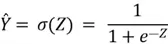
To understand the relevance of this sigmoid function, let’s inspect its shape below:

The linear equation function above that produces is an unbounded function. This means that the linear function can produce any real number such that can take up any value in the range . However, since probabilities by definition can only be between 0 and 1, we need an additional function that can ‘squish’ the values between to a much smaller range of (0, 1). This is where the sigmoid function comes into play. Inspecting its graphed form above, we can see that as increases, the function steadily approaches 1, and as decreases, the function approaches 0.

Furthermore, although it is not clear in the graph above, at , the value of the sigmoid function is precisely 0.5. Thus, if , will be less than 0.5, which will produce a prediction of ‘0’ (the negative class). On the other hand, if turns out to be positive, will be greater than 0.5, which creates a prediction of ‘1’ or the positive class. This is our decision boundary.

Cost Function and Gradient Descent in Logistic Regression

Now that we know how a Logistic Regression classifier estimates probabilities and generates predictions, the question is again about how the model is trained to find the optimal set of parameters.

Recall our discussion about the cost functions and gradient descent in the previous tip about Linear Regression. The purpose of the cost function is to create a measure that defines how well our model performs. Although accuracy is one way to measure this performance. We can define more robust and differentiable loss functions better, such as the binary cross entropy (BCE) loss:

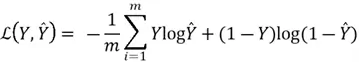
Where is the total number of training examples, is the real label, and is the estimated probability.

The reason why Mean Square Error (MSE) is not suitable here is because of the different nature of output in regression tasks versus classification tasks. Furthermore, MSE is a non-convex function that can create optimization challenges during gradient descent as it has multiple local minima. This can lead gradient descent to settle in suboptimal solutions. This is not the best possible optimal solution as shown below:

BCE Loss

On the other hand, the BCE loss is carefully constructed with certain properties. In case of a mismatch of prediction, e.g., if is 0.12 but is 1, the BCE loss is designed to give a high loss. On the contrary, if is close to , the prediction is rewarded with low cost. The most robust feature of this loss function is that it rewards or penalizes a prediction based on how far or close it is to the actual true label. For instance, for , a of 0.3 will receive a much higher loss associated with it, as compared to a of 0.4. Furthermore, it is differentiable and convex, which ensures an optimal solution being found by the gradient descent algorithm.

Algorithm Steps

Fortunately for the gradient descent algorithm, the steps are identical with the algorithm used in Linear Regression. Below are the steps:

1. We randomly initialize the parameters of our model.
2. The gradient of the cost function with respect to parameters is then computed. Through calculus, the gradients can be computed as:

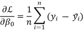
3. Once we have these gradients, we can update the parameters using the following formula:

Note: If the gradient is negative, we will be adding to the value of and thus increasing it. If the gradient is positive, we will be subtracting from the , and thus decreasing it.

here is the learning rate. It is a hyperparameter that controls the size of the step we are taking towards the minimum of our MSE function. If is very small, it will take very long to reach the minimum point. On the other hand, if is very large, we can potentially miss the minimum and fail to converge. Therefore, we need to find an appropriate value of alpha through hyperparameter tuning. We will be exploring this later with K-Fold Cross Validation.

4. We repeat steps 2 and 3 until the BCE stabilizes and does not decrease much further.

Logistic Regression Algorithm

Now that we have all the tools in place, we can summarize the entire pipeline for the Logistic Regression model:

1. Define the Model Equation: This process involves identifying the relevant features in your dataset, and establishing the following equation:

2. Define the Cost Function: To find the best-fit line, we need a way to measure how well our model fits the data. For this purpose, we will be using BCE:

3. Apply Gradient Descent to Minimize the Cost Function: We will optimize our cost function to find our model parameters that yield the smallest BCE on the training dataset. For each parameter, the update rule is:

4. Make Predictions: Once we have identified the best fitting decision boundary for our dataset, we can use it to predict our test dataset and evaluate the performance using metrics like accuracy and F1 score.

K-Fold Cross Validation

K-Fold Cross-Validation is a systematic method to evaluate model performance. In the context of hyperparameter tuning, such as finding the optimal learning rate for a model , K-Fold Cross-Validation ensures that the evaluation is unbiased and reliable, thus allowing us to choose the best possible . For hyperparameter tuning of , we can employ the following steps with K-Fold Cross Validation:

Step 1

Choose a range of potential learning rates to test (e.g. 0.0001, 0.001, 0.01, 0.1). These learning rates can be specified manually or picked randomly, either uniformly or logarithmically, in a given range.

Step 2

Split the original training dataset into K subsets. For instance, if your training dataset has 10,000 observations and your fold size is 5. This means each subset will contain 20,000 observations after splitting.

Step 3

For each subset, one of them is reserved as the test set and the rest K-1 groups are kept as the training set. For each learning rate, a model is fit on this training set, and then evaluated on the test set. The performance is retained, and the model is discarded. This step is repeated k times with the same learning rate to ensure that every fold or subset has been used as a test set for evaluating. The model’s performance on each fold is averaged and noted down.

Step 4

Next, repeat Step 3 for another model with the next learning rate.

Step 5

When we have all the average scores for models with different learning rates, we can select the best model, and hence the best learning rate as the one with the best score. We can then train our model on the original dataset with the best learning rate found through K-Fold Cross Validation.

Implementing Logistic Regression in Python

In this part, we will be showing how to implement a Logistic Regression model from scratch, alongside a demonstration of hyperparameter tuning with K-Fold Cross Validation technique. For a practical demonstration, we will be using the Age Prediction Dataset to predict whether a particular person is an adult or a senior citizen. The dataset contains numerous features like respondent’s body mass index, blood glucose level after fasting, blood insulin levels, etc., to help the model make a decision. To get started on building our logistic regression model from scratch, we will first import the following libraries and packages:

#MSSQLTips.com (Python)
import pandas as pd
import numpy as np
import matplotlib.pyplot as plt
import seaborn as sns
from sklearn.metrics import accuracy_score
from sklearn.metrics import classification_report

Now, we can start reading our dataset into a dataframe to inspect it better.

#MSSQLTips.com (Python)
data = pd.read_csv('/content/age_predictions_cleaned.csv')
print("Shape: ", data.shape)
data.info()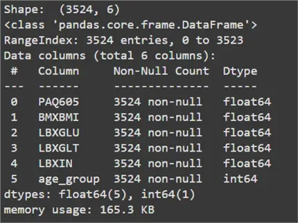

#MSSQLTips.com (Python)
data.head()

Data Analysis

From the output above, we can infer that the dataset consists of 3,524 total observations. These have a total of five features. The variable age_group is our target variable. A label of ‘0’ indicates an adult and a label of ‘1’ indicates a senior citizen. PAQ605 is the only categorical attribute in this dataset. A value of ‘1’ represents that the person takes part in weekly moderate or vigorous physical activity. A value of ‘2’ represents that they do not. For simplicity, we will be one-hot encoding this variable where ‘1’ indicates intensive physical activity and ‘0’ indicates sedentary activity.

#MSSQLTips.com (Python)
data['PAQ605'] = data['PAQ605'].replace(2.0, 0)

Now, we will be splitting our dataset into training and test sets. Since the dataset is rather small, we will be sampling 15% of the original dataset for the test set.

#MSSQLTips.com (Python)
train = data.sample(frac=0.85, random_state=200)
test = data.drop(train.index)
train.reset_index(drop=True, inplace=True)
test.reset_index(drop=True, inplace=True)
train = train.to_numpy()
test = test.to_numpy()

Logistic Regression Class

Our dataset is well prepared, so we can begin by creating a class for our Logistic Regression classifier.

#MSSQLTips.com (Python)
class LogisticRegression:
    def __init__(self, learning_rate=0.01, n_iterations=1000):
        """
        Initialize the logistic regression model.
        Parameters:
        - learning_rate: The learning rate for gradient descent.
        - n_iterations: The number of iterations for gradient descent.
        """
 
        self.learning_rate = learning_rate
        self.n_iterations = n_iterations
        self.weights = None
        self.bias = None
 
    def sigmoid(self, z):
        """
        Compute the sigmoid function.
        Parameters:
        - z: Linear combination of weights and inputs.
        Returns:
        - Sigmoid activation.
        """
 
        return 1 / (1 + np.exp(-z))
 
    def cross_entropy_loss(self, y_true, y_predicted):
        """
        Compute the cross-entropy loss.
        Parameters:
        - y_true: True labels.
        - y_predicted: Predicted probabilities.
        Returns:
        - Cross-entropy loss.
        """
 
        epsilon = 1e-15
        y_predicted = np.clip(y_predicted, epsilon, 1 - epsilon)
        n_samples = len(y_true)
        loss = -(1 / n_samples) * np.sum(y_true * np.log(y_predicted) + (1 - y_true) * np.log(1 - y_predicted))
        return loss
 
    def fit(self, X, y):
        """
        Fit the model to the data using gradient descent.
        Parameters:
        - X: Feature matrix (m samples x n features).
        - y: Target vector (m samples).
        """
 
        # Initialize parameters
        n_samples, n_features = X.shape
        self.weights = np.zeros(n_features)
        self.bias = 0
 
        loss_history = []
 
        # Gradient descent
        for i in range(self.n_iterations):
            # Linear model
            linear_model = np.dot(X, self.weights) + self.bias
            y_predicted = self.sigmoid(linear_model)
 
            loss = self.cross_entropy_loss(y, y_predicted)
            loss_history.append(loss)
 
            # Gradients
            dw = (1 / n_samples) * np.dot(X.T, (y_predicted - y))
            db = (1 / n_samples) * np.sum(y_predicted - y)
 
            # Update parameters
            self.weights -= self.learning_rate * dw
            self.bias -= self.learning_rate * db
 
            if i % 5000 == 0:
                print(f"Iteration {i}: Loss = {loss:.4f}")
        
        return loss_history
 
    def predict_prob(self, X):
        """
        Predict probability estimates for the input features.
        Parameters:
        - X: Feature matrix (m samples x n features).
        Returns:
        - Probabilities for each sample.
        """
 
        linear_model = np.dot(X, self.weights) + self.bias
        return self.sigmoid(linear_model)
 
    def predict(self, X):
        """
        Predict binary labels for the input features.
        Parameters:
        - X: Feature matrix (m samples x n features).
        Returns:
        - Binary labels (0 or 1).
        - Logit Probabilities. 
        """
 
        probabilities = self.predict_prob(X)
        label = np.where(probabilities >= 0.5, 1, 0)
        return probabilities, label

Begin Model Training

Now that we have a classifier coded up, we can initialize it and begin its training.

#MSSQLTips.com (Python)
model = LogisticRegression(learning_rate=0.0001, n_iterations=100000)
loss = model.fit(train[:, :-1], train[:, -1])

To visualize if the gradient descent is working correctly, we can plot the model’s loss per epoch, as shown below.

#MSSQLTips.com (Python)
plt.plot(range(len(loss)), loss, label='Loss')
plt.xlabel('Iterations')
plt.ylabel('Loss')
plt.title('Loss vs Iterations')
plt.legend()
plt.show()

Since the loss is steadily decreasing, we can be assured that our model works correctly.

Evaluate Model with Sklearn’s Classification Report Function

Now that our model is trained, let’s evaluate it using Sklearn’s classification report function.

#MSSQLTips.com (Python)
y_prob, y_pred = model.predict(test[:, :-1])
report = classification_report(test[:, -1], y_pred)
print(report)

From these results, we can see that the model has an accuracy and F1 score of 68%. This is not very desirable. To this end, we can try K-Fold Cross Validation to perhaps find a better learning rate. This will improve our model’s performance. For this step, we will be using a fold size of 5.

#MSSQLTips.com (Python)
alpha = [0.00001, 0.0001, 0.001, 0.01, 0.1, 1]
 
def kfold_cv(X, y, k=5, alpha=None):
    # Initialize the list to store cross-validation scores for each C
    cv_scores = {a: [] for a in alpha}
 
    # Split the data into k folds
    n_samples = len(X)
    fold_size = n_samples // k
    indices = np.arange(n_samples)
    np.random.shuffle(indices)
 
    # Perform cross-validation
    for a in alpha:
        # Initialize the logistic regression model with the current C
        print("Learning Rate:", a)
        model = LogisticRegression(learning_rate=a, n_iterations=100000)
 
        # Loop over each fold
        for i in range(k):
            # Create the validation set (the i-th fold)
            val_indices = indices[i * fold_size: (i + 1) * fold_size]
            train_indices = np.concatenate([indices[:i * fold_size], indices[(i + 1) * fold_size:]])
 
            X_train, X_val = X[train_indices], X[val_indices]
            y_train, y_val = y[train_indices], y[val_indices]
 
            # Fit the model on the training set
            model.fit(X_train, y_train)
 
            # Predict on the validation set
            prob, y_pred = model.predict(X_val)
 
            # Calculate accuracy and append to the list of scores
            score = accuracy_score(y_val, y_pred)
            cv_scores[a].append(score)
    # Return the average accuracy for each C
    avg_cv_scores = {a: np.mean(scores) for a, scores in cv_scores.items()}
    return avg_cv_scores
avg_cv_scores = kfold_cv(train[:, :-1], train[:, -1], k=5, alpha=alpha)

Plot Learning Rate

If we plot the accuracy for each learning rate, we get the plot below.

#MSSQLTips.com (Python)
plt.plot(list(avg_cv_scores.keys()), list(avg_cv_scores.values()), marker='o', linestyle='-', color='b')
plt.xscale('log')  # Log scale for C
plt.xlabel('Learning Rate')
plt.ylabel('Accuracy')
plt.title('K-Fold Cross Validation Results')
plt.grid(True)
plt.show()

Interpreting this plot, we can see that the best learning rate is 0.0001 as its corresponding accuracy is the highest among all the models.

Conclusion

This tip introduced the Logistic Regression classifier. We have reviewed and extensively explained the theory behind the fundamentals of this model. This includes its overall algorithm and training procedure. We then used a real-world survey dataset to train a classifier. The goal is to predict if a particular individual is a senior citizen based on several biomedical features. K-Fold Cross Validation technique was also demonstrated to introduce readers to the concept of hyperparameter tuning.

Next Steps

• Perhaps the most interesting revelation is the use of Logistic Regression for multiclass classification. To explore this concept further, readers can investigate one vs. one and one vs. all pipelines.
• Recall that Logistic Regression is a linear classifier. Since the model we implemented above did not perform very well, it is possible that the classes in the dataset used are non-linearly separable. Thus, readers are advised to look into data preprocessing and feature engineering techniques. These can aid in linearizing the class separability in the data.
• Another strength of Logistic Regression is that it offers interpretable results. This is the case for understanding how each feature influences the model’s predictions. Readers should explore how various visualization and coefficient analysis techniques can be utilized. They help to determine the predictive power of the dataset’s features.
• Other techniques relevant to hyperparameter tuning are:
  • Grid Search Cross Validation
  • Randomized Search Cross Validation
  • Bayesian Optimization
• Check out more AI related tips.

Harris Amjad

Harris Amjad currently works as a Software Engineer at Strategic Systems International. He is Microsoft Certified Data Analyst and Microsoft Certified Trainer. A rigorous, task-driven Data Enthusiast with substantial experience in Data Science, Data Analysis, and Data Engineering.

• MSSQLTips Awards: Trendsetter (25+ tips) – 2024 | Author Contender – 2023, 2024 | Rookie Contender – 2022