Problem
In this tip we will see how the attention mechanism has proven to be a breath of fresh air when working with complex language tasks as compared to its predecessors (like LSTMs and RNNs) by first seeing what problems it solves. Then, we will see what goes on behind the attention mechanism and the mathematical computations involved in generating accurate outputs. Finally, we will see the implementation of the attention mechanism in Python code.
Solution
The attention mechanism is one of the most important components of the Transformer architecture, that allows the model to pay attention to the most relevant parts of the input data when performing a task, similar to the way humans pay attention. The purpose of attention is simple: to allow the neural network to dynamically weigh the importance of different parts of the input data when processing any piece of data.
What happens behind the scenes?
To properly understand what goes on behind the attention mechanism and why it’s so revolutionary, let’s take a look the problems it solves, which were limitations of its predecessors (such as Recurrent Neural Networks and Long Short-Term memory models):
Capturing Long-Range Dependencies
In sequential tasks like language processing, a word’s meaning often depends on words that appeared much earlier in the sentence or paragraph. Before attention existed, older models struggled with this issue. For example, in the sentence: “The singer, after performing at a concert for three hours straight, was really tired”, when processing the word “tired”, the model needs to connect it back to “singer”. The necessary information had to go through many network layers, resulting in the information getting lost also known as the vanishing gradient problem.
With attention, a direct shortcut is created between the word “tired” and every word in the sentence, including “singer”. As a result, the model can instantly access the relevance of the earlier word in a sentence, ensuring the critical context is not lost.
Enabling Parallelization
RNNs are inherently sequential; meaning that they must process every word in order, one after the other. This makes them extremely slow to train on modern hardware, increasing computational overhead on the hardware which is optimized for parallel operations.
The attention mechanism eliminates this issue by computing the relationship between all words at the same time. This allows the entire input sequence to be processed at once, drastically improving the training time of the model.
Flexible Context Use
Rather than just passing a single fixed size context vector (like in the case of LSTMs), attention allows the model to create a unique context for every single output element. Let’s take the following Spanish sentence as an example: “Tengo una casa bonita” and translate it to: “I have a nice house”, the attention mechanism, when generating the English word “house”, can be trained to look mainly at the Spanish word “casa” and less at the other Spanish words, “Tengo”, “una”, or “bonita”. This highlights the ability of the attention mechanism to use a flexible weighted context tailored to the word it is currently producing.
The mathematical framework: Query, Key and Value
Now we know why the attention mechanism is so important to learn, let’s dive into the mathematical principles involved in the implementation of this technique.
Calculating attention requires three essential input vectors for every element in the sequence (for example, every word):
- Query (Q): This vector represents the current element we are focused on. It asks: “which element am I looking for?”
- Key (K): This vector represents the information that each token in the sentence “offers”. It’s what the query is compared against to establish similarity or relevance.
- Value (V): These vectors contain the actual content of all the elements that will be combined to form the final attended output.
The desired outcome is to compute an output vector that is a weighted sum of the Value vectors, where the weights are determined by how much is each Key relevant to the Query.
The Calculations
Firstly, we start off by calculating the alignment score between the Query (Q) and the Key (K) by using the dot product like so:
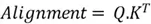
Here, ![]() means the transpose of the Key (K) matrix. An important thing to note is that the larger the magnitude of the alignment score means a higher similarity and a greater relevance.
means the transpose of the Key (K) matrix. An important thing to note is that the larger the magnitude of the alignment score means a higher similarity and a greater relevance.
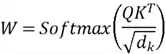
This dot product is then scaled using the square root of the dimension of the key vectors like ![]() . This step prevents the score from becoming too large and pushing the softmax function into regions where it has tiny gradients, making the softmax function difficult to learn.
. This step prevents the score from becoming too large and pushing the softmax function into regions where it has tiny gradients, making the softmax function difficult to learn.
After these 2 steps comes the normalization by passing the result ![]() through a softmax function to transform them into probabilities, which have a value ranging from 0 to 1. These are known as the attention weights:
through a softmax function to transform them into probabilities, which have a value ranging from 0 to 1. These are known as the attention weights:
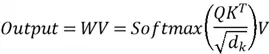
Finally, these attention weights are multiplied by their corresponding Value (V) vectors and are summed up to produce the final context vector (or output) as shown below:
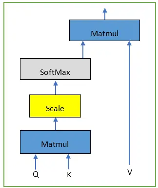
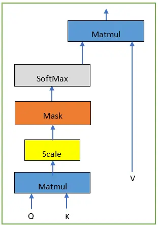
The diagram showing the mathematical framework involved in the attention layer is shown below:
Understanding the mathematical computation
To understand this mathematical computation a bit more in detail, let’s take a look at an example.
Let’s consider the sentence “I love running” with the embedding vectors:
I ![]()
Love ![]()
Running ![]()
We will first transform these individual embedding vectors into an input vector ![]() , which we will use to create our Query (Q), Key (K) and Value (V) matrices:
, which we will use to create our Query (Q), Key (K) and Value (V) matrices:
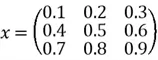
It’s important to remember that every row in the matrix is the embedding vector of every word in order as present in the sentence. Since the length (or dimension) of each embedding vector is 3, we can say that ![]()
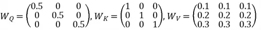
Next, we will move on to creating our Q, K and V matrices by first assuming values for the weight matrices ![]() ,
, ![]() and
and ![]() as given below.
as given below.
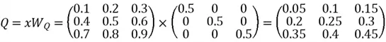
We calculate Q by:
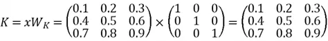
Calculate K by:
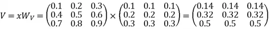
We calculate V by:
Now that we have our Q, K and V vectors, it’s time to compute the attention weights W like so:
The transpose of the K vector 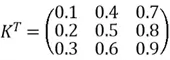
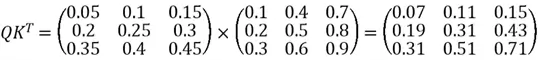
The dot product of the Q and ![]() (alignment score) will be calculated as:
(alignment score) will be calculated as:
As we have the embedding dimension ![]() , we will scale the dot product above like so:
, we will scale the dot product above like so:
Scaled scores 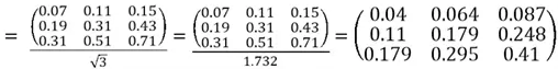
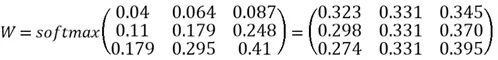
Finally, W will be calculated as:
Now that we have got our W matrix, we will multiply this result with the V vector to generate the output matrix, where each row is a context-aware representation of the input embedding matrix x:

Types of attention
At this point, we have explored the mathematical side of the attention mechanism and its significance in modern day deep learning applications. But did you know that there are multiple versions of the attention layer that exist? Let’s take a look at them.
Self-Attention
This type of attention is the most common and powerful one, being used in the transformer’s encoder. The three vectors come from the same input source (say, a sentence being processed). As a result, a word is able to find contextual relationships within its own sentence.
Masked Self-Attention
This is used exclusively in the transformer’s decoder during the training phase. Similar to self-attention (shown in the diagram below), but masking (a technique which involves adding the ![]() product with a matrix with 0s and numbers approaching negative infinity) is applied to the similarity scores, preventing a word from “looking ahead” at words that come later in the sequence like so:
product with a matrix with 0s and numbers approaching negative infinity) is applied to the similarity scores, preventing a word from “looking ahead” at words that come later in the sequence like so:

This mode of operation preserves the autoregressive nature needed for generation of the current sequence element output.
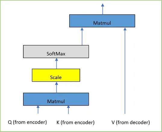
Cross-Attention
Here, the Query matrix comes from the target sequence (Decoder output), and the Key and Value matrices come from the source sequence (Encoder output). This will allow the decoder to focus on the parts of the input which are the most relevant for generating the output. This technique is commonly utilized to connect two different sequences (e.g. during a language translation consist of a source language and a target language).
The diagram illustrating this type of attention mechanism can be seen below:
Multi-Headed Attention
At this point, we now how different types of attention work in the transformer architecture. But one might think: why do we need multiple heads if one can take care of the sequence?
Let’s consider an example of a single flashlight trying to illuminate the important parts of a sentence. But a sentence will have various kinds of relationships to understand, such as subject-verb, object-pronoun, adjective-noun, and long-range dependencies. Instead of one head handling all these different relationships, it would be prudent to give the model multiple heads, each focusing on a different relationship in a sentence. This is known as multi-head attention.
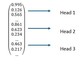
Therefore, we split the embeddings into smaller parts and run multiple attention heads in parallel, with each head independently working on each relationship as shown below.
At the end of the computation for each head, the outputs are concatenated and projected back to the original embedding size.
Python Demo
We will now implement what we have learned so far in this tip in Python by considering a different example.
Firstly, we will import the numpy library as well as initialize the embedding dimension and the input sequence: “The singer, after performing at a concert for three hours straight was really tired”.
#MSSQLTips.com (Python)
#Importing numpy
import numpy as np
#1. Define d_k (dimension of the vectors)
d_k = 4
# 2. Input Sentence (Tokenized form)
tokens = ["The", "singer", ",", "after", "performing", "at", "a", "concert", "for", "three", "hours", "straight", ",", "was", "really", "tired"]
We will take a random initialization of the Query vector, focusing on the last word “tired”. This vector will ask: “what is the reason behind being tired?”. Similarly, the Key vectors pertaining to the word “tired” will represent the person/subjects involved:
#MSSQLTips.com (Python)

Q_tired = np.array([5.0, 1.0, 0.5, 0.0])
K_singer = np.array([4.8, 1.2, 0.4, 0.1]) # High match to Q
K_concert = np.array([2.0, 0.0, 0.0, 0.0]) # Medium match (relevant event)
K_hours = np.array([1.5, 0.8, 0.1, 0.0]) # Medium match (relevant duration)
K_irrelevant = np.array([0.1, 0.1, 0.1, 0.1]) # Low match (e.g., "The")
# Combine all keys into a matrix (K_matrix)
K_matrix = np.stack([K_singer, K_concert, K_hours, K_irrelevant])
For simplicity, we will calculate attention scored against these four key vectors.
The value matrix will contain the content that will be summed up after computing the attention scores between Q and K and is initialised like so:
#MSSQLTips.com (Python)
V_singer = np.array([9.0, 1.0, 0.0, 0.0])
V_concert = np.array([0.0, 0.5, 1.0, 0.0])
V_hours = np.array([0.0, 0.1, 0.5, 1.0])
V_irrelevant = np.array([0.1, 0.0, 0.0, 0.0])
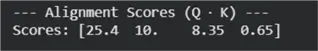
V_matrix = np.stack([V_singer, V_concert, V_hours, V_irrelevant])Now, we will calculate the alignment scores:
#MSSQLTips.com (Python)

scores = np.dot(Q_tired, K_matrix.T)
print("--- Alignment Scores (Q · K) ---")
print(f"Scores: {scores}")
The output of this code block will be:
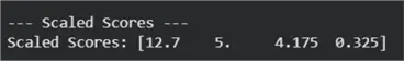
This attention score will be scaled as shown below:
#MSSQLTips.com (Python)

scale_factor = np.sqrt(d_k)
scaled_scores = scores / scale_factor
print("\n--- Scaled Scores ---")
print(f"Scaled Scores: {scaled_scores}")
The output of this code will be:
After applying softmax to these scores, we will get the following result:
#MSSQLTips.com (Python)

def softmax(x):
    e_x = np.exp(x - np.max(x)) # Subtract max for numerical stability
    return e_x / e_x.sum(axis=0)

attention_weights = softmax(scaled_scores)
print("\n--- Attention Weights (SoftMax) ---")
print(f"Weights: {attention_weights}")
From the vector above, we see that “Singer” gets ~99.95% of the attention, correctly linking “tired” to the subject.
Finally, we will compute the output vector for the word “tired”:
#MSSQLTips.com (Python)

Z_tired = np.dot(attention_weights, V_matrix)

print("\n--- Final Attention Output Vector (Z) ---")
print(f"Output Vector (Z): {Z_tired}")
From the result above, we can conclude that the word “tired” receives 99.93% of its context from the word “singer”.
Conclusion
To summarize, we have seen how the attention mechanism has become the fundamental backbone of modern deep learning application. We started off by looking at why the attention is great at what it does, and the essential components that constitute it, namely the query, key and value vectors. Here, we saw how they are used in scaled dot-product attention to generate attention scores, integral for deducing contextual relationships between words in a sequence. After this we saw the various types of attention used in the encoder and decoder stacks and covered its code implementation to give a hands-on experience. Congrats! Now you know what’s needed to understand one of the major parts of the Transformer.
Next Steps
- For more curious readers, they should try implementing a harder example having a longer sentence as an input to the attention mechanism and setting a larger embedding dimension for the vectors to see how powerful the attention mechanism is.
- Instead of a language translation task, one could try text summarization as well to see the attention mechanism work in a different capacity.
- To checkout more AI related tips.

Harris Amjad currently works as a Software Engineer at Strategic Systems International. He is Microsoft Certified Data Analyst and Microsoft Certified Trainer. A rigorous, task-driven Data Enthusiast with substantial experience in Data Science, Data Analysis, and Data Engineering.
- MSSQLTips Awards: Trendsetter (25+ tips) – 2024 | Author Contender – 2023, 2024 | Rookie Contender – 2022