Introduction to Machine Learning with Neural Networks – Part 3

Problem

Now that we are familiar with a variety of supervised learning models, we arrive at the meat of Machine Learning. Neural networks are one of the most powerful and widely used machine learning algorithms today, especially for complex tasks like image recognition and natural language processing. However, for a beginner, the mathematical details and concepts, such as layers, weights, and activation functions, may seem daunting. This tip aims to introduce Neural Networks in a simplified manner to help beginners understand how they work and how they can be applied at a very basic level.

Solution

During this past decade and especially in our current digital landscape, anyone even faintly familiar with the field of machine learning and artificial intelligence recognizes the term ‘Neural Networks’. To someone unfamiliar with the workings of a Neural Network, it might feel like an abstract and mystical piece of technology, something that is very powerful but extremely difficult to grasp, or just a fancy buzzword for others. This tip will attempt to clear this ambiguity and haze around Neural Networks, especially for beginners who want to dive deeper into how these Neural Network models work, and discover how they are used and their legacy and relevance in the current AI realm.

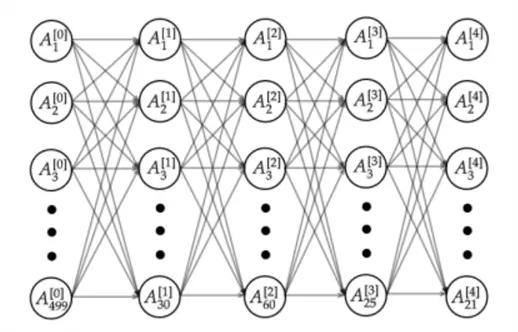
Neural Networks are essentially the building block of deep learning, becoming a fundamental model from which more advanced models like convolutional neural networks (CNN) and recurrent neural networks (RNN) are built. In more precise mathematical theory, Neural Networks are thought of as universal approximators that can estimate any continuous function or mapping given enough neurons and proper training. In layman’s terms, this means that the architecture of Neural Networks is capable of learning any non-linear and complex relationship between data, whether it’s predicting stock prices, recognizing faces, or translating languages. These models do not need a specific formula, but just enough data to learn patterns from examples.

Basic Structure of Neural Network

Before diving deeper into Neural Networks, we must first understand their basic structure and some common terminology associated with it.

Recall the logistic regression classifier shown below. It takes in four features that are then multiplied with their respective weights. A bias term is then added before passing the value through an ‘activation function’ like sigmoid to produce the output.

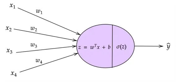
In the context of a Neural Network, the logistic regression classifier can be thought of as a single neuron of the network–the basic unit of a Neural Network. So, if we stack multiple interconnected logistic regression units across several layers, we get a Neural Network like the one below.

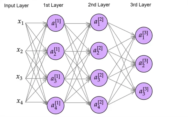
A Neural Network like the one above is comprised of several key components, each playing a specific role in how the network learns and makes predictions.

Neurons

As mentioned previously, this is a basic unit of a Neural Network with a similar structure to that of a logistic regression unit. It takes the input and applies algebraic manipulation with weights and bias before passing the result to an activation function.

Layers

Neurons are generally grouped across different layers. For instance, in the diagram above, there are 4 neurons present in the 1st layer. On the other hand, represents a third neuron in the 2nd layer of the network.

The input layer of the network comprises the input features being passed into the network. Notice that each neuron in the 1st layer is connected with all the input neurons. Generally, such Neural Networks, where every neuron in a layer is connected to every neuron in the previous layer, are termed fully connected Neural Networks. ‘Connected’ here means that output from one neuron is being passed as an input to another neuron.

Furthermore, the 1st and 2nd layers are termed the hidden layers, as these are intermediate layers and we don’t observe the output of these layers directly. The 3rd layer is our output layer. The 3-layer Neural Network shown above has 3 neurons in the output layer. This could perhaps indicate that we are working with a multiclass classification setting where the goal is to predict three classes (e.g., whether an image is that of a cat, dog, or bird).

The number of hidden layers and the number of neurons per layer is a hyperparameter, and a near-optimal value can be determined using techniques like grid search or cross-validation.

Weights and Bias

These are our model parameters that the model attempts to learn while training to help map a function between the input and the output layer. The concept is similar to the one described in logistic regression and linear regression; however, the number of parameters is exorbitantly more in Neural Networks. Each connection between neurons has a weight, and in fully connected layers, every neuron connects to every neuron in the next layer.

So, if we do a bit of math for our Neural Network above:

• Since there are 4 neurons in the 1st layer, with each neuron connected to each of the four input features, we get total weights in the 1st layer.
• Similarly, in the 2nd layer, there are 4 neurons, each connected to all of the 4 neurons of the 1st layer. This again produces weights.
• In the 3rd layer, there are 3 neurons, each connected to all of the 2nd layer’s 4 neurons. This requires neurons.

When we sum these weights up from each layer, we get a total of 44 weights! Even the very small Neural Network above has a large number of weights. This is one reason why Neural Networks are highly powerful at capturing complex relationships due to the flexibility given by a huge number of weights.

Activation Function

These functions determine the output of a neuron and help introduce nonlinearity in the network. Sigmoid is one activation function you are likely familiar with. It allows us to project the weighted sum of inputs between 0 to 1, to stimulate probability scores in a logistic regression classifier. Although sigmoid function is used in Neural Networks, particularly in the output layer if we are dealing with binary classification tasks, a range of other functions also exist, like , , and . Each of them has its pros and cons. is commonly used, particularly amongst the hidden layers as it is computationally inexpensive. It can be considered as one of the model’s hyperparameters.

Forward and Backward Pass

Now that we are familiar with some basics associated with Neural Networks, let’s try to understand how the model makes predictions and learns its weights.

Neural Networks learn by passing the data forward through the network to make predictions. Then, a loss function evaluates this prediction, comparing it with the actual ground truth value. Lastly, the model learns from its mistakes and adjusts its parameters value. The steps of this entire process are forward pass, evaluation, and then backward pass. We will attempt to understand these processes using our example 3-layer Neural Network discussed and illustrated previously.

It is also important to note that Neural Networks rely heavily on matrix operations for efficient computations since we are dealing with several features, and perhaps millions of data points at once. Here are some important matrices to take note of:

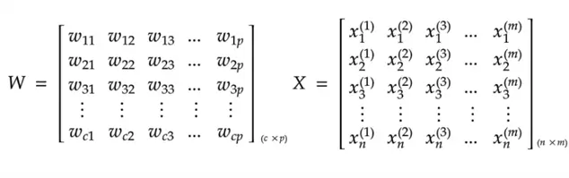
Let’s go over these matrices one by one:

• is a weight matrix with a dimension . Each layer of the Neural Network will have its own unique weight matrix. Coming back to the dimension of this matrix, is the number of neurons in the current layer, and is the number of neurons in the previous layer of the network.

Recall that for our example Neural Network, the number of weights required for our 1st layer was 16. Also, recall that the number of neurons in the 1st layer was 4 and the number of neurons in the previous input layer was 4. Therefore, the weight matrix for this network’s first layer should have the dimension which amounts to a total of 16 weight elements within the matrix.

Although it is understandably hard to visualize what is being multiplied by what, let’s consider the element in the matrix. It simply represents the weight connecting the first neuron in a layer with the previous layer’s first neuron. In short, is the value of the output from the previous layer’s first neuron will be multiplied by to produce the output for the current layer’s first neuron.

• is our dataset in matrix form. It has a dimension of where is the number of features in the dataset and is the total number of observations.

Now that we understand some basic matrix notation, let’s move forward to understanding the Neural Network’s predictions and learning process. For simplicity, we are assuming we are working with a dataset of 4 features and total observations.

Forward Pass

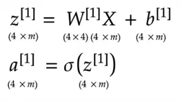
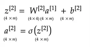
Forward propagation involves getting the output by passing the input through each layer. In the first layer, the input dataset is multiplied by the weight matrix and then a bias is added, before the resulting vector is passed through an activation function. This produces this layer’s output, which becomes the input for the next layer, and the process repeats until we are at the output layer. Here’s a mathematical demonstration of this process using our 3-layer Neural Network:

1st Layer:

2nd Layer:

3rd Layer:

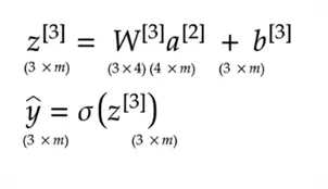
It is essential to make sure that the shape of the matrices aligns for matrix multiplication.

Evaluation

Once we have a prediction by our Neural Network, it is time to evaluate it with an adequate loss function. If we are working with a classification task, a cross-entropy loss is typically used. Otherwise, for regression-related tasks, mean square error loss may also be used. The details and peculiarities of these different loss functions have been discussed in previous tips.

Backward Pass

Now comes a slightly complicated concept. Recall that in logistic regression, we updated the model parameters by computing the derivatives of the weights. Here, we will employ the same technique for Neural Networks, except that now we are required to compute derivatives of each weight across each and every layer. Although we won’t be delving into the entire derivation of these gradients as it requires a strong grasp of calculus, here are some important equations to note:

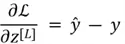
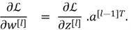
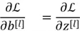
Once we have computed the gradients of parameters in the backward propagation, we can employ gradient descent and update the parameters accordingly.

The Neural Network Algorithm

Now that we have some intuition behind the working of a Neural Network, let’s summarize the steps of its algorithm below:

1. Forward Pass: The input passes through layers of the network, and is transformed by the weights, bias, and activation functions to produce an output in the last layer of the network.
2. Evaluation: The prediction by the network is evaluated using a loss function.
3. Backward Pass: Gradients are computed for each parameter in the network in a sequential manner.
4. Parameters Update: The parameters are then updated using the update rule we have used previously:

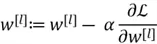
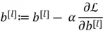
Where is the learning rate.

Implementation in Python

Now that we have gone over the theory of Neural Networks, it is time to understand and implement them practically. For this reason, we will revisit the MNIST digit classification dataset and attempt to solve the problem through Neural Networks. Since there is little benefit to implementing Neural Networks from scratch, we will instead employ Scikit-learn, TensorFlow, and PyTorch to aid us. These are some of the most robust libraries and frameworks in Python that provide Machine Learning engineers with efficient, scalable, and production-ready solutions.

Libraries Needed

To get started, we first need to import the following libraries and modules:

#MSSQLTips.com (Python)
#required libraries
import pandas as pd
import numpy as np
 
from sklearn.neural_network import MLPClassifier
from sklearn.metrics import classification_report
from sklearn.metrics import confusion_matrix
 
import tensorflow as tf
from tensorflow import keras
from tensorflow.keras import layers
 
import torch
import torch.nn as nn
import torch.optim as optim
from torch.utils.data import TensorDataset, DataLoader

Read Dataset

Then, let’s read the dataset into a dataframe and inspect its dimensions.

#MSSQLTips.com (Python)
#reading dataset
train = pd.read_csv("/content/mnist_train.csv")
test = pd.read_csv("/content/mnist_test.csv")
#shape of Dataset
print("Shape of train: ", train.shape)
print("Shape of test: ", test.shape)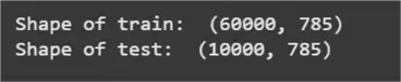

From the output above, this is a pretty large dataset with 60,000 data points in the train dataset and 10,000 data points in the test dataset. Both data frames share 785 columns. Let’s inspect this dataset directly as well.

#MSSQLTips.com (Python)
#displaying the train dataset
train.iloc[:, :20].head()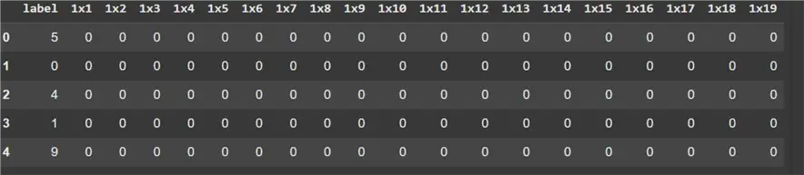

As observed above, this is a very sparse dataset with many zero entries. This is not, however, surprising as each column denotes a pixel value, which can take any value between 0 to 255. Since the edges of a digit image are likely to be blank, it might explain why the initial values in the dataset are all zero. Furthermore, we can also observe a label column representing the digit written in an image.

Moving on, it is good practice to be familiar with the spread and distribution of the features of our dataset. We can use Pandas inbuilt functions to display this information.

#MSSQLTips.com (Python)
#descriptive Stats
train.describe()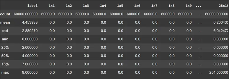

It is also good practice to visualize the class distribution of our dataset. In case of a heavy imbalance, we might need to take additional steps to minimize the model’s bias towards the majority class.

#MSSQLTips.com (Python)
#class Distribution
train['label'].value_counts()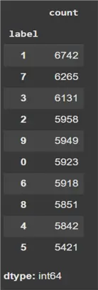

Fortunately, that dataset is almost uniform in terms of the class distribution of the label column, which means we do not have to make any changes to this dataset to deal with class imbalance. As we can see above, most of the digits have roughly the same number of data points.

Additional Data Preprocessing

Before we can implement and train a Neural Network model, we must perform some additional data preprocessing. First, labels and features must be split and stored in separate dataframes as shown below.

#MSSQLTips.com (Python)
#splitting labels from features
X_train = train.iloc[:, 1:]
Y_train = train.iloc[:, 0]
X_test = test.iloc[:, 1:]
Y_test = test.iloc[:, 0]
 
print("Shape of X_train: ", X_train.shape)
print("Shape of Y_train: ", Y_train.shape)
print("Shape of X_test: ", X_test.shape)
print("Shape of Y_test: ", Y_test.shape)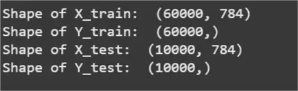

Second, we need to normalize the features. This process involves scaling the features from their current range to an interval of [0,1]. Since the features of this dataset comprise pixel values that can take any value between 0-255, we divide each column by 255 to project the features to 0-1 range. This step helps to train the model much faster.

#MSSQLTips.com (Python)
#normalizing features
X_train = X_train/255
X_test = X_test/255

Train Neural Network

We can now train our Neural Networks to predict digits from image-based data. First, we will be employing Scikit-learn, a simple and efficient machine learning library in Python for classical ML algorithms, including support for Neural Networks via the ‘MLPClassifier’ module as demonstrated below.

#MSSQLTips.com (Python)
#sklearn neural network
sk_NN = MLPClassifier(hidden_layer_sizes=(128, 64), activation='relu', solver='adam', verbose=True, random_state=42, max_iter=50)
sk_NN.fit(X_train, Y_train)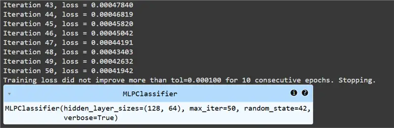

From the code above, we can infer that this Neural Network has two hidden layers–one with a size of 128 neurons and the other with 64 neurons. The output layer is determined automatically by the package, and it has 10 neurons, as we have 10 digits in our dataset as seen before. Thus, we are training a 3-layer Neural Network. We have also specified RELU as the activation function, with a total of 50 iterations of training. We are also employing an advanced and better version of gradient descent, called Adam’s optimizer, for training this model.

Once our model is trained, we can predict the test dataset and evaluate the model’s performance. The result for Scikit-learn’s Neural Network model is shown below. As you can see, we have achieved an impressive result of 98% accuracy on the MNIST test dataset.

#MSSQLTips.com (Python)
#predicting test dataset
y_pred = sk_NN.predict(X_test)
print(classification_report(Y_test, y_pred))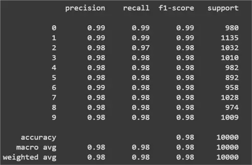

Moving forward, we will now introduce frameworks and libraries preferred by industry and research experts in their daily machine learning related tasks. First is TensorFlow, a powerful open-source deep learning framework by Google, optimized for large-scale Neural Networks and GPU acceleration. As we can see below, TensorFlow makes it easy to build very complex networks.

#MSSQLTips.com (Python)
#tensorFlow neural network
tf_NN = keras.Sequential([
    layers.Dense(128, activation='relu', input_shape=(784,)), #First hidden layer (128 neurons)
    layers.Dense(64, activation='relu'),                      #Second hidden layer (64 neurons)
    layers.Dense(10, activation='softmax')                    #Output layer (10 classes for digits 0-9)
])
 
tf_NN.compile(optimizer='adam', 
              loss='sparse_categorical_crossentropy', 
              metrics=['accuracy'])
 
tf_NN.fit(X_train, Y_train, epochs=50, batch_size=10000, validation_data=(X_test, Y_test))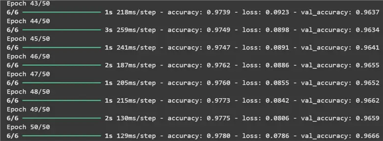

We have specified somewhat of the same Neural Network as the one we trained using Scikit-learn. The hidden layers, number of neurons, total iterations, and optimizer remain the same. However, a new hyperparameter might be the ‘batch_size’ parameter within the ‘fit()’ function. This refers to the number of data points processed before the weights of the network are updated.

Predicting using this network, we once again get an impressive stat of about 97% accuracy.

#MSSQLTips.com (Python)
#predicting test dataset
loss, accuracy = tf_NN.evaluate(X_test, Y_test)
print("Accuracy: ", accuracy)

Using PyTorch

Last, we will briefly cover PyTorch, a flexible deep learning framework by Meta, known for dynamic computation graphs, ease of debugging, and strong GPU support. Although the syntax of PyTorch is very similar to TensorFlow, there are some minor changes. For once, in PyTorch, Neural Networks expect data in the form of tensors and need efficient data loading mechanisms.

#MSSQLTips.com (Python)
#pytorch neural network
 
#conversion from np to tensor
X_train_tensor = torch.tensor(X_train.to_numpy(), dtype=torch.float32)
X_test_tensor = torch.tensor(X_test.to_numpy(), dtype=torch.float32)
Y_train_tensor = torch.tensor(Y_train.to_numpy(), dtype=torch.long)  
Y_test_tensor = torch.tensor(Y_test.to_numpy(), dtype=torch.long)
 
#create tensordataset object
train_dataset = TensorDataset(X_train_tensor, Y_train_tensor)
test_dataset = TensorDataset(X_test_tensor, Y_test_tensor)
 
#dataloader pipeline
train_loader = DataLoader(train_dataset, batch_size=32, shuffle=True)
test_loader = DataLoader(test_dataset, batch_size=32, shuffle=False)

Only after completing this step can we specify the Neural Network architecture and begin training the model.

#MSSQLTips.com (Python)
#pytorch model
 
class model(nn.Module):
    def __init__(self):
        super(model, self).__init__()
        self.fc1 = nn.Linear(784, 128) #First hidden layer (128 neurons)
        self.fc2 = nn.Linear(128, 64)  #Second hidden layer (64 neurons)
        self.fc3 = nn.Linear(64, 10)   #Output layer  (10 neurons)
        self.relu = nn.ReLU()          #Activation function
    
    def forward(self, x):
        x = self.relu(self.fc1(x))
        x = self.relu(self.fc2(x))
        x = self.fc3(x)  #No activation (logits)
        return x
py_NN = model()
loss = nn.CrossEntropyLoss()  
optimizer = optim.Adam(py_NN.parameters(), lr=0.0001)
 
#training model
py_NN.train()
for epochs in range(50):
  total_loss = 0.0
  for x, y in train_loader:
 
    optimizer.zero_grad()
    output = py_NN(x)
    loss_value = loss(output, y)
    loss_value.backward()
    optimizer.step()
 
    total_loss += loss_value.item()
 
  avg_loss = total_loss / len(train_loader)
  print(f"Epoch {epochs + 1}/{50}, Loss: {avg_loss}")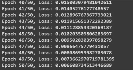

With the model trained, we can finally evaluate it. Once again, we get accuracy of around 97.5%, which is very similar to our previous models. This is hardly surprising as we employed the same hyperparameters and model architecture across all three frameworks.

#MSSQLTips.com (Python)
#model evaluation
py_NN.eval()
correct_pred = 0
total_pred = 0
 
with torch.no_grad():
  for x, y in test_loader:
    output = py_NN(x)
    predictions = output.argmax(dim=1)
    correct_pred += (predictions == y).sum().item()
    total_pred += y.size(0)
 
accuracy = correct_pred / total_pred
print(f"Accuracy: {accuracy}")

Although it is entirely possible to code from scratch the same Neural Networks that we have trained above, it will be a very daunting task, prone to errors and computational inefficiencies. These frameworks, on the other hand, save time, improve efficiency, and enable training on GPUs with minimal code!

Conclusion

In this tip, we explored the fundamentals of Neural Networks, breaking down their core components, theoretical foundations, and mathematical basics. We examined how these models process information, learn patterns, and make predictions. Beyond theory, we provided a hands-on demonstration of how to build and train a Neural Network using three powerful frameworks: Scikit-learn, TensorFlow, and PyTorch. Each framework offers unique advantages, catering to different levels of complexity and use cases.

Next Steps

Congratulations if you have come to this point and understood most of the information. You have come a long way in understanding Neural Networks, and for those who wish to further improve their understanding and foundations of deep learning, here are a couple of recommendations:

• If the reader wishes to understand backpropagation in depth, they should try implementing a simple Neural Network from scratch. This will not only help to refine the reader’s programming skills but also enhance the understanding of the model’s learning process.
• Secondly, knowing how a Neural Network works is often not enough. The design of a Neural Network can be thought of as a recipe that should have the perfect amount of ingredients. This involves carefully choosing the number of layers, the number of neurons, the learning rate, the batch size, which activation function to choose, etc.
• For the most interested readers, they can also look into the weaknesses of Neural Networks and how that motivated the development of other advanced variations of this model.
• Also, check out more AI related tips on MSSQLTips.com.

Harris Amjad

Harris Amjad currently works as a Software Engineer at Strategic Systems International. He is Microsoft Certified Data Analyst and Microsoft Certified Trainer. A rigorous, task-driven Data Enthusiast with substantial experience in Data Science, Data Analysis, and Data Engineering.

• MSSQLTips Awards: Trendsetter (25+ tips) – 2024 | Author Contender – 2023, 2024 | Rookie Contender – 2022