Problem
Time series datasets often arrive in one of two structural formats: long or wide.
In a long format, each row represents a single observation for a specific entity at a specific timestamp value. At a minimum, this structure includes three columns: an entity identifier (such as a product name, stock ticker, or weather station), a timestamp identifier, such as hourly, daily, weekly, or monthly time periods), and the observed value. While time periods may repeat across entities, the combination of entity and timestamp values uniquely identifies each row of a long format dataset.
In contrast, a wide format organizes time series data horizontally. Each row in a timestamp column corresponds to a unique time period, and each column beyond the timestamp identifier represents a different observation type, such as diameter, thickness, and smoothness for silicon and silicon carbide computer chips. This data structure is potentially more performant than a long format because it can store the same amount of data in substantially fewer rows.
This tip focuses on computing EMAs from source data in a wide format, using recursive CTEs. A prior tip (Note to MSSQLTips.com Editor: please add an anchor for “Calculating Exponential Moving Averages in SQL Server Using CTEs and Stored Procedures” that is still in queue to be published) explored the same EMA logic using a long format structure. By comparing these approaches, readers can better understand the trade-offs in performance, clarity, and lifecycle safety when modeling time series data in SQL Server.
Solution
Moving averages can filter (or smooth) random variations in time series data. The two most common moving averages are the Simple Moving Average (SMA) and the Exponential Moving Average (EMA). When recent values need to be weighted more heavily—such as in financial analytics or safety monitoring—EMAs are preferred. Safety monitoring and financial analytics are similar in that they can both benefit by responding to early warning signs.
This tip’s first substantive section presents selected excerpts from a time series dataset in a long format, followed by a short T-SQL script that transforms it into a wide format. This transformation helps clarify the structural differences and sets the stage for comparing EMA processing logic across formats.
The second section walks through recursive CTE logic for computing three EMA sets—based on 21-, 50-, and 200-period lookback windows—for a single ticker. It also demonstrates how to join these EMA sets into a unified result, a common practice in financial analytics to assess directional movement.
The third section compares EMAs calculated for the same time series data formatted alternatively in both long and short formats. The code in this section demonstrates how to calculate, manipulate, and display underlying time series data, EMAs, and metadata parameters.
The Data for This Tip
Data for this tip derives from a prior tip “Static Versus Dynamic Bulk Insert Imports of Multi-File Datasets”. The data in the ticker_date_price table, which is excerpted in the following four screenshots, is in a long format. It has three ticker values (SPY, DIA, IWM).
- The ticker column is for entity values.
- The date column is for timestamp values.
- The beginning timestamp value is different for each ticker because the underlying security for each ticker was initially offered for sale on different dates.
- The ending timestamp value is the same for all three tickers because that is the last date for which observations were made.
- The price column contains observation values for the ticker and date column values on each row.
- The ticker_date_price table has a primary key based on ticker and date column values in ascending order.
- There are four screenshots depicting selected sets of ten rows each.
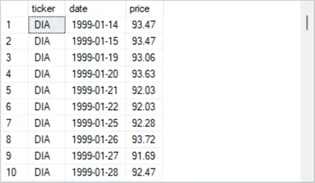
- The first excerpt shows the first ten rows for the DIA ticker. The first row for the DIA ticker has a timestamp value of 1999-01-14.
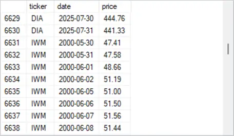
- The second excerpt shows the two most recent rows for the DIA ticker with timestamp values of 2025-07-30 and 2025-07-31 followed by the first eight rows for the IWM ticker. The first row for the IWM ticker has a timestamp value of 2000-05-30.
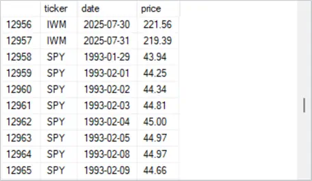
- The third excerpt shows the two most recent rows for the IWM ticker with timestamp values of 2025-07-30 and 2025-07-31 followed by the first eight rows for the SPY ticker. The first row for the SPY ticker has a timestamp value of 1993-01-29.
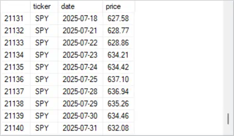
- The fourth excerpt shows the last ten rows for the SPY ticker. The last row, which is the most recent row for the SPY ticker, has a timestamp value of 2025-07-31. The row indicator in last row of the ticker_date_price table reveals that the count of rows for the table is 21140.
T-SQL Script
The following script includes T-SQL code for transforming the ticker_date_price table in a long format to a wide format table named widepricetable.
- A use SSMS statement sets the default database for the script to the [T-SQLDemos] database.
- Next, a drop table statement conditionally removes a table named widepricetable.
- Then, the first select statement transforms the arrangement of values from a long format in the ticker_date_price table to a wide format in a table named widepricetable. Conditional aggregation statements (max case when…) perform the pivot and renames the pivoted column values to spy_price, dia_price, and iwm_price, respectively.
- The last select statement displays all the column values of the table named widepricetable.
use [T-SQLDemos];

-- pivot a long format table in dbo.ticker_date_price
-- to a wide format table in dbo.widepricetable

drop table if exists dbo.widepricetable;

-- pivot code for transforming a long format layout to a wide format layout
select
    date,
    max(case when ticker = 'SPY' then price end) AS spy_price,
    max(case when ticker = 'DIA' then price end) AS dia_price,
    max(case when ticker = 'IWM' then price end) AS iwm_price
into dbo.widepricetable
from dbo.ticker_date_price
group by date
order by date;

-- display dbo.widepricetable
select *
from dbo.widepricetable
order by date
Data Output
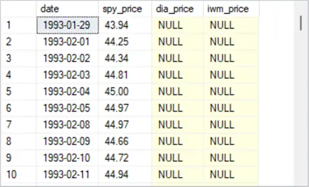
The following screenshot shows the first ten rows from the table named widepricetable.
- The first row has a date column value of 1993-01-29.
- All ten rows in the spy_price column are populated with prices, but the first ten rows of the dia_price and iwm_price columns contain null values. This is because the underlying security for the SPY ticker was launched years before the underlying securities for both the DIA and IWM tickers.
Additional Data
The next screenshot shows the last ten rows from the table named widepricetable.
- All ten rows in spy_price, dia_price, and iwm_price columns have non-null price values. Furthermore, the values in the spy_price column below perfectly match the price column values for the last set of rows in the ticker_date_price table.
- The screenshot below illustrates another benefit of a wide format table. For example, you can tell by casual observation that SPY prices increase from the first through the last trading day in the excerpt. In contrast, the other two tickers do not have their prices increase over the same timeframe. Because the long format table layout does not show side-by-side observation values across tickers on the same dates, users of the long format table will require some custom programming to tell if prices grow for SPY but not for both DIA and IWM.

Recursive EMA Logic for SPY Across Multiple Period Lengths
This section provides a high-level overview of the recursive CTE logic for computing Exponential Moving Averages (EMAs) for the SPY ticker using three common lookback windows: 21, 50, and 200 periods. A lookback window is alternatively referred as a period length. These EMA sets are computed independently and then optionally merged into a unified result set for comparative analysis. This approach illustrates how analysts assess directional movement by comparing closing prices to EMAs of varying period lengths.
Recursive CTEs allow you to compute EMAs one day (or any time period) at a time using iterative logic—without relying on while loops or cursors. Recursive CTEs aren’t just for finance. Whether you’re smoothing sales trends, replenishing inventory, or modeling temperature shifts, the same logic applies. Wherever time series data needs smoothing to reveal trends, recursive CTEs offer a modular approach that can be readily implemented within SQL Server.
T-SQL Script
The following script has four main sections. The first three populate temporary tables for EMA values that are based on three distinct lookback windows (21, 50, and 200). Within each section, an initial EMA value is calculated based on the length of the lookback window. This initial EMA is the simple moving average across the underlying values in the initial lookback period, and it is what comments in the code refer to as the lifecycle gate. Next, recursive calculations are applied for computing EMA values based on the current period’s underlying entity attribute (price) and the EMA value for the preceding period. The weights for the inputs to the current period’s EMA value are based on the period lengths. The shorter the period length, the greater the weight is for the current period’s underlying price relative to the EMA value for the prior period. The final script section optionally merges the three EMA value sets into a global temporary table (##spy_ema_wide).
use [T-SQLDemos];

-- Compute ema value sets for spy ticker
-- Step 1: Compute Scalar SMA Seed for spy EMA_21

drop table if exists #spy_sma21_seed;

select avg(spy_price) as spy_sma21_seed
into #spy_sma21_seed
from (
    select top 21 spy_price
    from widepricetable
    where spy_price is not null
    order by date
) as seed_window;

-- Step 2: Recursive EMA_21 for spy with Lifecycle-Aware Start
drop table if exists #spy_ema21;

with base as (
    select date, spy_price, row_number() over (order by date) as rn
    from widepricetable
    where spy_price is not null
),
seed as (
    select spy_sma21_seed from #spy_sma21_seed
),
ema_cte as (
    -- Seed EMA_21 at row 21 using the SMA
    select
        b.rn,
        b.date,
        b.spy_price,
        cast(s.spy_sma21_seed as float) as spy_ema21
    from base b
    cross join seed s
    where b.rn = 21

    union all

    -- Recursively compute EMA_21 from row 22 onward
    select
        b.rn,
        b.date,
        b.spy_price,
        cast(0.0909 * b.spy_price + 0.9091 * e.spy_ema21 as float)
    from base b
    join ema_cte e on b.rn = e.rn + 1
)
select * into #spy_ema21 from ema_cte option (maxrecursion 0);

-- optionally display #spy_ema21 values set
-- select * from #spy_ema21

---------------------------------------------------------------------

-- Compute #ema_50 values set

-- Step 1: Compute Scalar SMA Seed for spy EMA_50
drop table if exists #spy_sma50_seed;

select avg(spy_price) as spy_sma50_seed
into #spy_sma50_seed
from (
    select top 50 spy_price
    from widepricetable
    where spy_price is not null
    order by date
) as seed_window;

-- Step 2: Recursive EMA_50 for spy with Lifecycle-Aware Start
drop table if exists #spy_ema50;

with base as (
    select date, spy_price, row_number() over (order by date) as rn
    from widepricetable
    where spy_price is not null
),
seed as (
    select spy_sma50_seed from #spy_sma50_seed
),
ema_cte as (
    -- Seed EMA_50 at row 50 using the SMA
    select
        b.rn,
        b.date,
        b.spy_price,
        cast(s.spy_sma50_seed as float) as spy_ema50
    from base b
    cross join seed s
    where b.rn = 50

    union all

    -- Recursively compute EMA_50 from row 51 onward
    select
        b.rn,
        b.date,
        b.spy_price,
        cast(0.0392 * b.spy_price + 0.9608 * e.spy_ema50 as float)
    from base b
    join ema_cte e on b.rn = e.rn + 1
)
select * into #spy_ema50 from ema_cte option (maxrecursion 0);

-- optionally display #spy_ema50 values set
-- select * from #spy_ema50

---------------------------------------------------------------------

 -- Compute #ema_200 values set

-- Step 1: Compute Scalar SMA Seed for spy EMA_200
drop table if exists #spy_sma200_seed;

-- compute the scalar seed value for spy_ema200
select avg(spy_price) as spy_sma200_seed
into #spy_sma200_seed
from (
    select top 200 spy_price
    from widepricetable
    where spy_price is not null
    order by date
) as seed_window;

-- this identifies the correct date to start the recursion
-- Identify the lifecycle gate date for spy EMA_200
drop table if exists #spy_seed200_date;

select top 1 date into #spy_seed200_date
from (
    select date, row_number() over (order by date) as rn
    from widepricetable
    where spy_price is not null
) as ranked
where rn = 200;

-- Step 2: Recursive EMA_200 for spy with Lifecycle-Aware Start
drop table if exists #spy_ema200;

-- Step 1: Build ranked base
with ranked_base as (
    select date, spy_price, row_number() over (order by date) as rn
    from widepricetable
    where spy_price is not null
),
seed as (
    select avg(spy_price) as spy_sma200_seed
    from (
        select top 200 spy_price
        from ranked_base
        order by rn
    ) as seed_window
),
ema_cte as (
    -- Seed EMA_200 at rn = 200
    select
        b.rn,
        b.date,
        b.spy_price,
        cast(s.spy_sma200_seed as float) as spy_ema200
    from ranked_base b
    cross join seed s
    where b.rn = 200

    union all

    -- Recursively compute EMA_200 from rn = 201 onward
    select
        b.rn,
        b.date,
        b.spy_price,
        cast(0.0100 * b.spy_price + 0.9900 * e.spy_ema200 as float)
    from ranked_base b
    join ema_cte e on b.rn = e.rn + 1
)
select * into #spy_ema200 from ema_cte option (maxrecursion 0);

-- optionally display #spy_ema200 values set
-- select * from #spy_ema200

-----------------------------------------------------------------------

-- optional merge for all three spy ema value sets into a single
-- wide-format temp table
drop table if exists ##spy_ema_wide;

select
    e21.date,
    e21.spy_price,
    e21.spy_ema21,
    e50.spy_ema50,
    e200.spy_ema200
into ##spy_ema_wide
from #spy_ema21 e21
left join #spy_ema50 e50 on e21.date = e50.date
left join #spy_ema200 e200 on e21.date = e200.date
order by e21.date;

select * from ##spy_ema_wide order by date;
Data Output
Here are the first ten rows from the merged result set.
- The spy_ema21 row value for 1993-03-01 is the seed EMA value, which is the simple moving average for the first twenty-one spy_price values from widepricetable.
- The spy_ema21 row value for 1993-03-02 is the first calculated EMA value based on the current spy_price value and the prior spy_ema21 value; this iterative process is repeated for all subsequent rows in widepricetable.
- The null column values for spy_ema50 and spy_ema200 are not populated in the first ten rows of the spy_ema21 column.

Here are the last ten rows from the merged result set.
- Notice that these ten rows have non-null EMA values for spy_ema21, spy_ema50, and spy_ema200 columns.
- In addition, the spy_ema21 column values are systematically closer to the spy_price column values. In fact, the greater the period length of the EMA column values, the more different the EMA column values are from the spy_price column values. In other words,
- the spy_ema200 column values are the most smoothed EMA column values,
- the spy_ema50 column values are less smoothed than the spy_ema200 column values, and
- the spy_ema21 column values are the least smoothed EMA column values.

Comparing EMAs Based on Long Versus Wide Underlying Data Formats
The prior sections of this tip describe a process for calculating EMAs for underlying data in a wide format. The “Calculating Exponential Moving Averages in SQL Server Using CTEs and Stored Procedures” tip shows how to process the same data when they are arranged in a long format. This section shows how to manipulate and compare the merged result set from this tip with the result set from the “A Stored Procedure for Calculating Emas Based on a SMA Seed Value” section in the “Calculating Exponential Moving Averages in SQL Server Using CTEs and Stored Procedures” tip.
The current tip calculates a single result set for a single dataset. For each run of the code in this tip, the contents of the merged result set (##spy_ema_wide) is freshly calculated based on the current source data. No history of EMA value sets or their source data is maintained. For the prior tip, the code framework maintains history of successively calculated EMA value sets and their source data (dbo.ticker_ema_history_from_sma_seed). The rows from each successive run of the code to calculate EMA value sets along with their underlying values are tagged with a run_timestamp column value that indicates when the calculations were started.
Since there are just three EMA value sets calculated in this tip, each of these sets is compared to corresponding EMA value sets from the most recent runtime value in the prior tip. This comparison presents side-by-side results from both the current tip and the prior tip. Three select statements extract data from dbo.ticker_ema_history_from_sma_seed for the prior tip and ##spy_ema_wide for the current tip. Because the current tip’s underlying prices and EMAs are derived from a global temporary table created in the preceding section, you may need to re-run the script in that section before extracting values with the following three select statements.
T-SQL Code
The code for each of the three comparisons appears below.
- The code for the first comparison is for EMA values with a period length of 21.
- The code for the second comparison is for EMA values with a period length of 50.
- The code for the third comparison is for EMA values with a period length of 200.
use [T-SQLDemos]

-- compare long-format EMA values with wide-format EMA values
-- for ticker = SPY and @period = 21

declare @period int = 21;
select
    l.date,
    cast(l.price as dec(5,2)) [spy_price from long format],
    cast(l.ema as dec(9,2)) [spy_ema21 from long format],
    w.spy_price [spy_price from wide format],
    cast(w.spy_ema21 as dec(9,2)) [spy_ema21 from wide format],
    @period as [period length],
    --w.spy_ema50,
    --w.spy_ema200,
    (2.0 / (@period + 1)) as [current value weight],
    (1.0 - (2.0 / (@period + 1))) as [prior ema weight]
from dbo.ticker_ema_history_from_sma_seed l
join ##spy_ema_wide w on l.date = w.date
where l.ticker = 'SPY'
  and l.period = @period
  and l.run_timestamp = (
      select max(l.run_timestamp)
      from dbo.ticker_ema_history_from_sma_seed l
      where l.ticker = 'SPY'
        and l.period = @period
  )
order by date;

-----------------------------------------------------------------

-- compare long-format EMA values with wide-format EMA values
-- for ticker = SPY and @period = 50

set @period = 50;

select
    l.date,
    cast(l.price as dec(5,2)) [spy_price from long format],
    cast(l.ema as dec(9,2)) [spy_ema50 from long format],
    w.spy_price [spy_price from wide format],
    cast(w.spy_ema50 as dec(9,2)) [spy_ema50 from wide format],
    @period as [period length],
    --w.spy_ema50,
    --w.spy_ema200,
    (2.0 / (@period + 1)) as [current value weight],
    (1.0 - (2.0 / (@period + 1))) as [prior ema weight]
from dbo.ticker_ema_history_from_sma_seed l
join ##spy_ema_wide w on l.date = w.date
where l.ticker = 'SPY'
  and l.period = @period
  and l.run_timestamp = (
      select max(l.run_timestamp)
      from dbo.ticker_ema_history_from_sma_seed l
      where l.ticker = 'SPY'
        and l.period = @period
  )
order by date;

-----------------------------------------------------------------

-- compare long-format EMA values with wide-format EMA values
-- for ticker = SPY and @period = 200

set @period = 200;

select
    l.date,
    cast(l.price as dec(5,2)) [spy_price from long format],
    cast(l.ema as dec(9,2)) [spy_ema200 from long format],
    w.spy_price [spy_price from wide format],
    cast(w.spy_ema200 as dec(9,2)) [spy_ema200 from wide format],
    @period as [period length],
    --w.spy_ema200,
    --w.spy_ema200,
    (2.0 / (@period + 1)) as [current value weight],
    (1.0 - (2.0 / (@period + 1))) as [prior ema weight]
from dbo.ticker_ema_history_from_sma_seed l
join ##spy_ema_wide w on l.date = w.date
where l.ticker = 'SPY'
  and l.period = @period
  and l.run_timestamp = (
      select max(l.run_timestamp)
      from dbo.ticker_ema_history_from_sma_seed l
      where l.ticker = 'SPY'
        and l.period = @period
  )
order by date;
Data Output
Here are excerpts of the first eight rows from each select statement in the preceding script.
- The period length column indicates the period length for each set of rows.
- The [spy_ema21 from long format], [spy_ema50 from long format] , and [spy_ema200 from long format] column values show the calculated EMA values for period lengths of 21, 50, and 200 in the prior tip. The source data for these calculations are in a long format.
- The [spy_ema21 from wide format], [spy_ema50 from wide format] , and [spy_ema200 from wide format] column values show the calculated EMA values for period lengths of 21, 50, and 200 period lengths from the current tip. The source data for these calculations are in a wide format.
- The [current value weight] and [prior ema weight] columns across all three table sections show how EMA responsiveness shifts with period length. Shorter lookback windows react faster to current period underlying values. Longer lookback windows place a greater emphasis on historical EMA values.
- The main take-away from these comparisons is that the EMA values for each period length are the same no matter whether the underlying source data are in a long or a wide format. Additionally, my casual observation was that the long format required a longer time to return EMA value sets.

Next Steps
This tip drills down on how to calculate EMA value sets based on different period lengths for time series datasets. The next best step for adding EMA computational techniques to your own toolset is to adapt the code in this tip to data that is available within your organization. Filtering time series data is a widely respected way of discerning changes in time series data over a collection of time periods. Recall that while this tip demonstrates the calculation of EMA value sets for financial securities, EMAs can provide valuable insights for time series data from any domain.
If you would like a more definitive study of how long it takes and the overall resource utilization for computing EMA values based on long versus wide datasets, please leave a comment with that request. I look forward to replying to that request with a follow-up tip.

Rick Dobson is a SQL Server professional with decades of T-SQL experience that includes authoring books, running a national seminar practice, working for businesses on finance and healthcare development projects, and serving as a regular contributor to MSSQLTips.com. He has been a practicing Python developer for more than the past half decade – with a special emphasis for data visualization and ETL tasks with JSON and CSV files. His most recent professional passions include financial time series data and analyses, AI models, and statistics. If you are interested in growing your skills in any of these areas especially as they relate to financial securities, consider visiting his blog at https://securitytradinganalytics.blogspot.com/2023/12/.
- MSSQLTips Awards: Leadership (200+ tips) – 2025 | Author of the Year Contender – 2017-2024