Problem
Hardware sensors or diverse types of equipment can generate IoT data at a high frequency, e.g., every second. Additionally, IoT data can be messy, semi-structured or just have huge volume and many disparate sources. How to ingest and model IoT data in Microsoft Fabric using the medallion lakehouse architecture?
Solution
The medallion architecture is an approach used to organize data in three different layers, where each layer builds progressively and incrementally on the previous one to provide a high-quality and reliable data product. This approach is not reserved for a single domain; data developers can apply it universally to build robust data products. Therefore, we can employ medallion architecture to clean and prepare IoT data for analytics in MS Fabric.
Sample data
To illustrate this scenario, we will use IoT data from a weather tracking system:
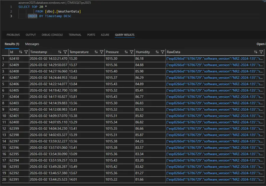
The sensor takes a new reading with a frequency of every 145 seconds and writes the data to the database. These data currently reside on an Azure SQL Server.
Create workspace
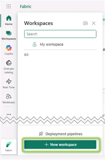
The first step is to head over to app.fabric.microsoft.com. From the Fabric homepage, select Workspaces, then New workspace:
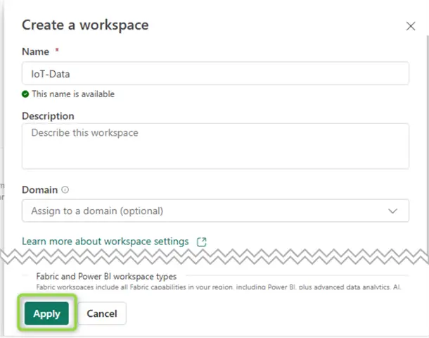
Give your workspace a name and hit Apply:
Create lakehouse
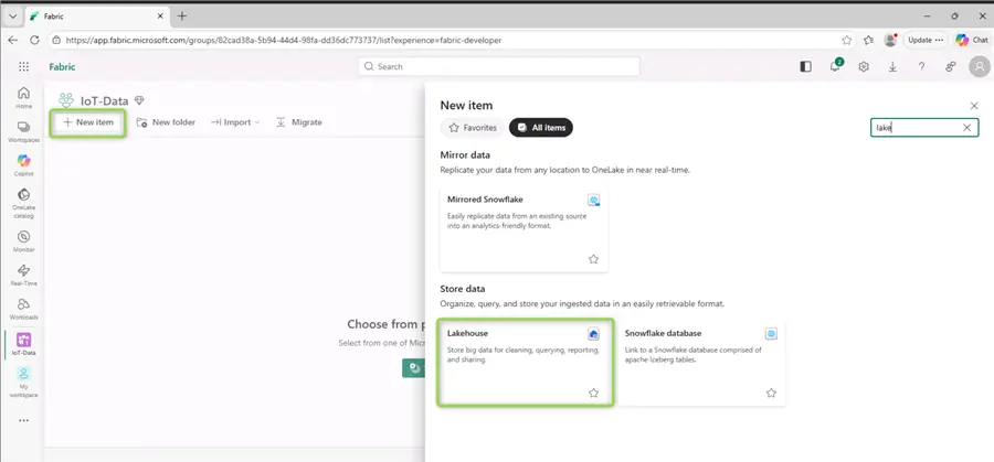
Next, from the home page of the newly created workspace, click New Item. Use the search bar to look for Lakehouse:
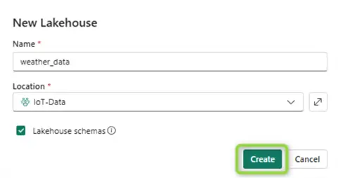
Give your new lakehouse a name and click Create:
Get data
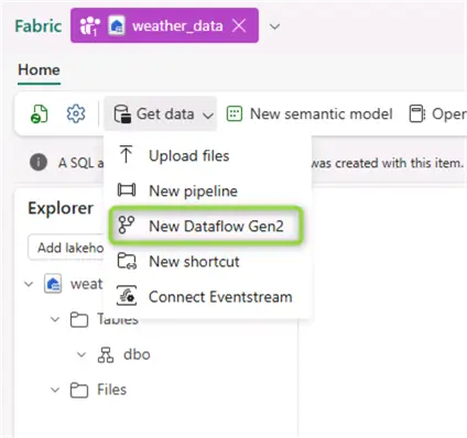
The next step is to get some data rolling into our newly created lakehouse. From the Get data menu, select New Dataflow Gen2:
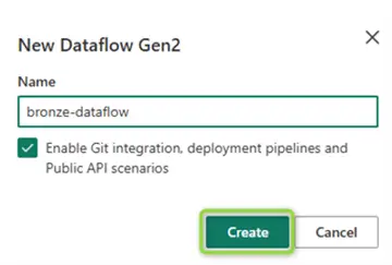
Give your new dataflow a name and click Create:
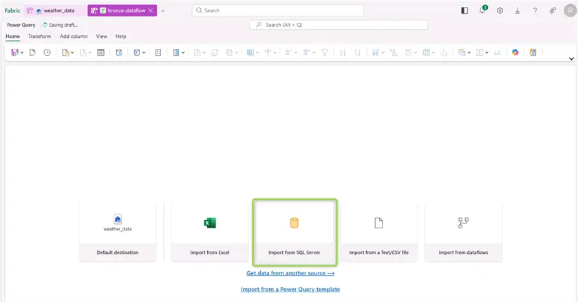
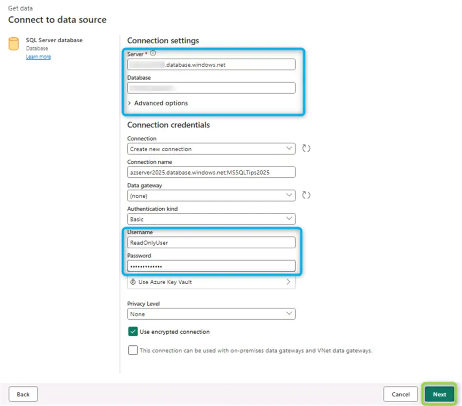
Now we have a blank dataflow. The first action point is to import data. We will use Azure SQL as the data source:
The data source connection pop-up will open, where we must provide connection details to our database:
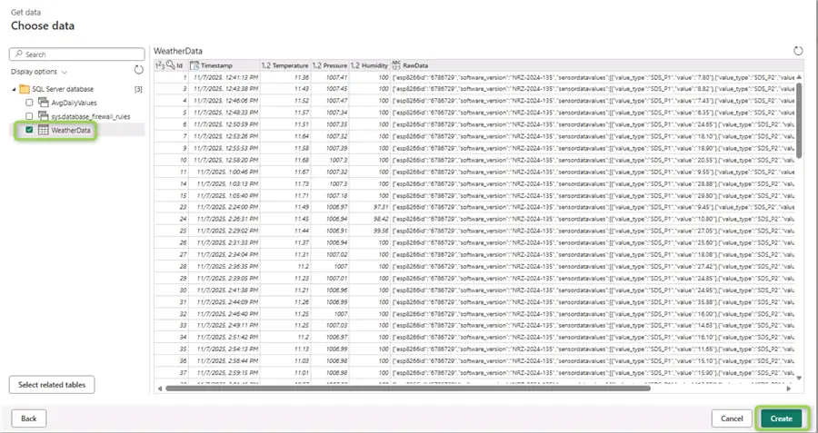
Once the dataflow establishes a connection to the database, we can see the object browser. We are interested in the WeatherData table:
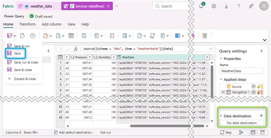
After clicking Create from the object browser, the Power Query editor view opens. You can use the Save button to make a quick save (in Blue, used to save the settings so far). Then from the bottom left-hand corner click the “+” next to Data destination. Note sometimes Fabric assigns directly the existing lakehouse as data destination. In any case, we need to reconfigure some stuff:
Bronze layer
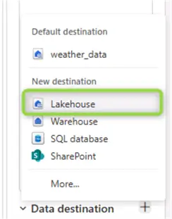
At this stage we begin the creation and configuration of the bronze layer. Choose Lakehouse from the Data destination section layer:
On the next screen, adjust the connection if needed:
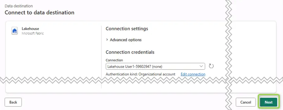
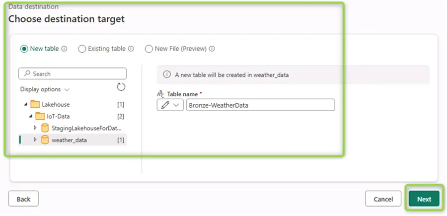
Then, you must select a container and give your new table a name:
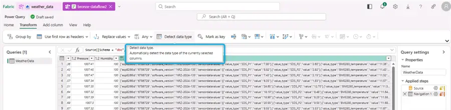
After clicking Next, the Power Query editor re-opens. Double-check if Power Query automatically selected the correct data types. Notice the RawData column, which is type JSON in SQL Server. It is a clever idea to use the Detect data type functionality and explicitly cast it to string:
If this column remains of type Any, we will not be able to include it in the destination:
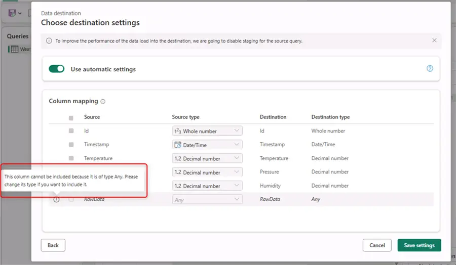
Additionally, toggle Use automatic settings to off. Then select Fixed schema under Schema options on publish. This important setting will allow the configuration of incremental refresh later, which is beneficial for frequently arriving IoT data. With incremental refresh we will be able to pick up only a certain number of the most recent records instead of refreshing the whole dataset every time.
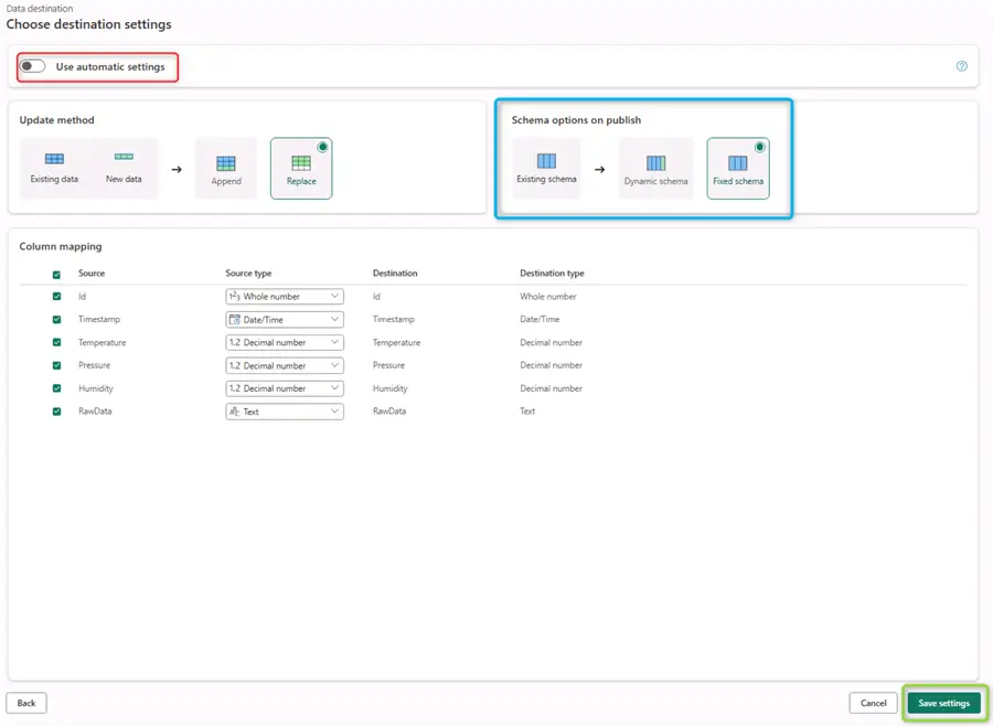
Everything looks fine so click Save Settings.
Configure incremental refresh
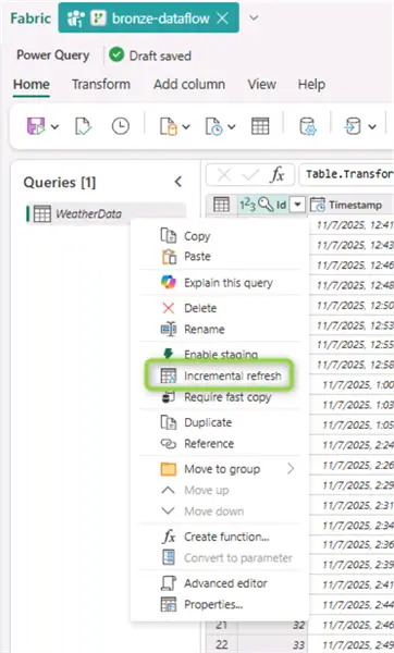
Back from the Power Query Editor, right-click on the WeatherData query, then click Incremental refresh:
The incremental refresh configuration pop-up will open:
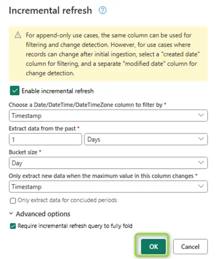
The smallest granularity is just a day. In our case this restricts subsequent loads to less than six hundred records every time the schedule triggers a refresh. To finish this part of the setup, click Save, run & close:
Configure automatic refresh
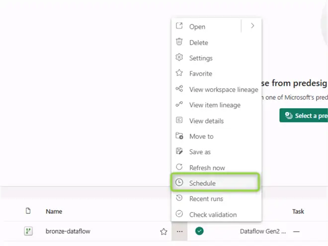
Back from the workspace homepage, you can find a list of your artifacts, at this point also including the data flow. Now we can schedule a regular refresh. Click on the three dots and select Schedule:
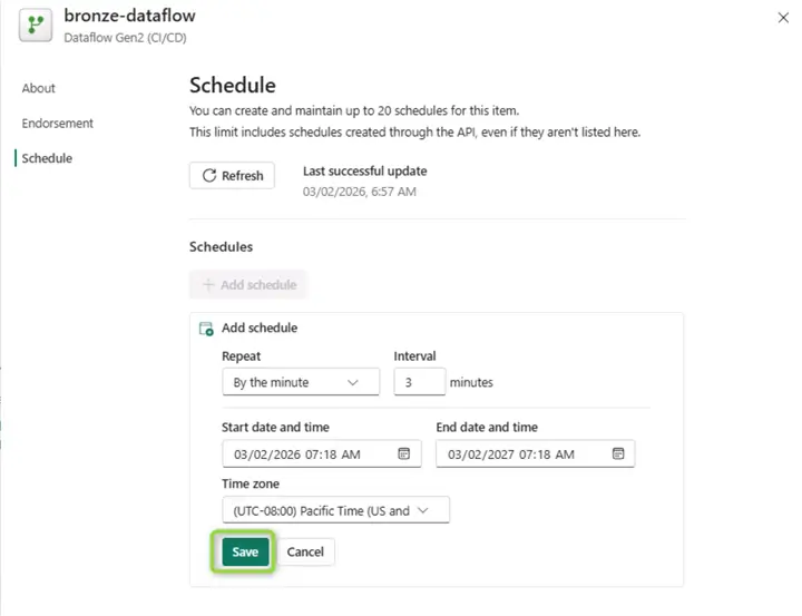
Then provide a suitable configuration and click Save:
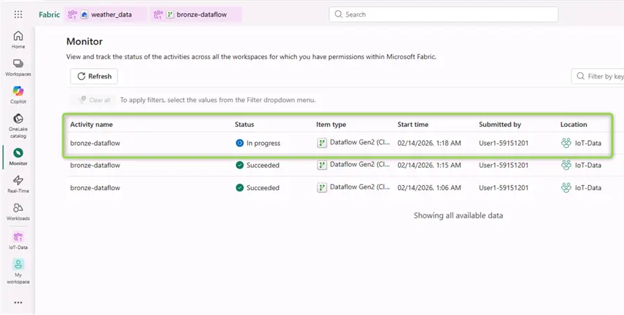
If we go to the Monitor tab, we can check the dataflow execution status of this and previous runs:
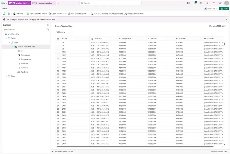
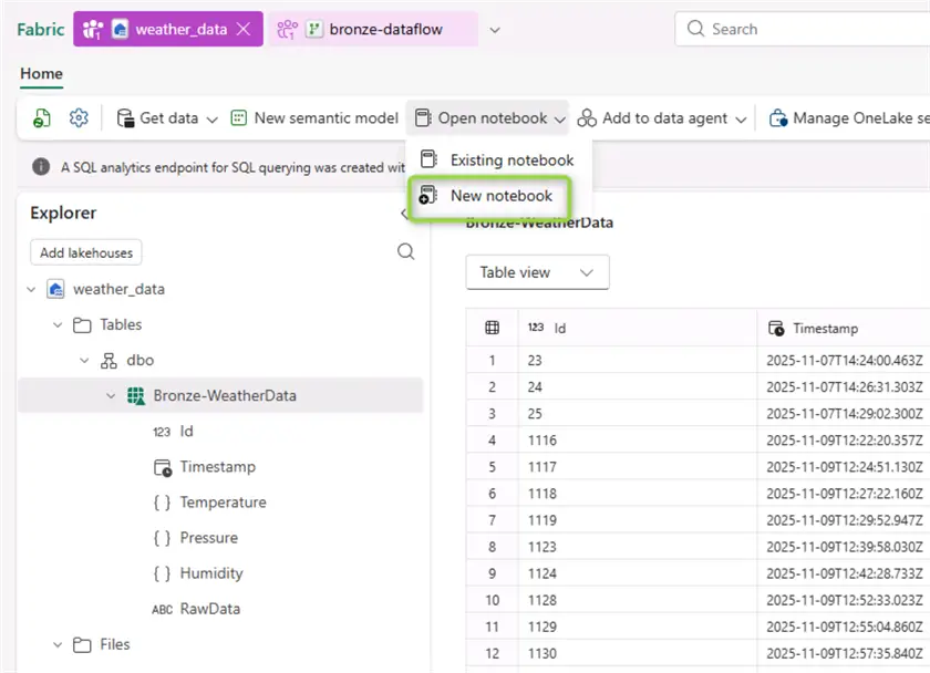
If the data was imported successfully, we can see our new delta table populated in the lakehouse. This is the bronze or raw data layer, therefore the data here are an exact replica of the source SQL data:
Silver layer
Create notebook
While viewing the contents of the bronze folder in your data lake, in the Open notebook menu, select New notebook:
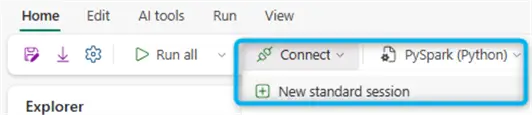
First, we need to start a new Spark session. Alternatively, the session will start automatically with the first code cell execution:
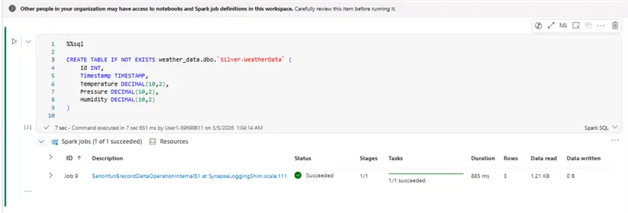
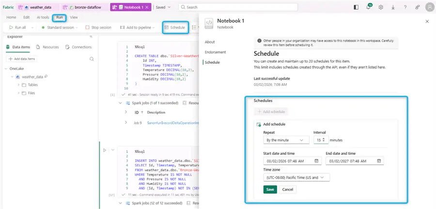
In the first code cell we will write Spark SQL code to create a new target table for the silver layer:
--MSSQLTips.com Spark SQL
%%sql
CREATE TABLE IF NOT EXISTS dbo.`Silver-WeatherData` (
Id INT,
Timestamp TIMESTAMP,
Temperature DECIMAL(10,2),
Pressure DECIMAL(10,2),
Humidity DECIMAL(10,2)
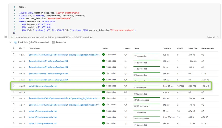
)In the second code cell we will define a query for appending new records from the bronze layer to the silver layer. The idea here is to filter out missing data and take only required columns:
--MSSQLTips.com Spark SQL
%%sql

INSERT INTO weather_data.dbo.`Silver-WeatherData`
SELECT Id
       , Timestamp
       , Temperature
       , Pressure
       , Humidity
FROM weather_data.dbo.`Bronze-WeatherData`
WHERE Temperature IS NOT NULL
  AND Pressure IS NOT NULL
  AND Humidity IS NOT NULL
  AND (Id, Timestamp) NOT IN (SELECT Id, Timestamp FROM weather_data.dbo.`Silver-WeatherData`)
You can monitor the output from the Spark job in the logs (just underneath each code cell). After a successful run we loaded over one hundred and twenty-seven thousand rows to the silver layer:
Schedule silver layer ingestion
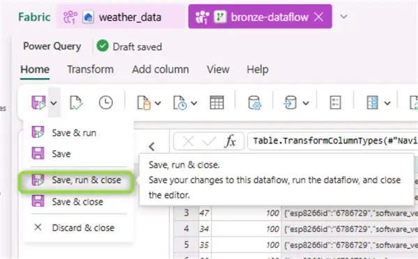
While still having the notebook open, from the Run tab we can use the Schedule menu to schedule the run of this notebook:
After scheduling the run, we are done with the silver layer.
Gold layer
Create notebook
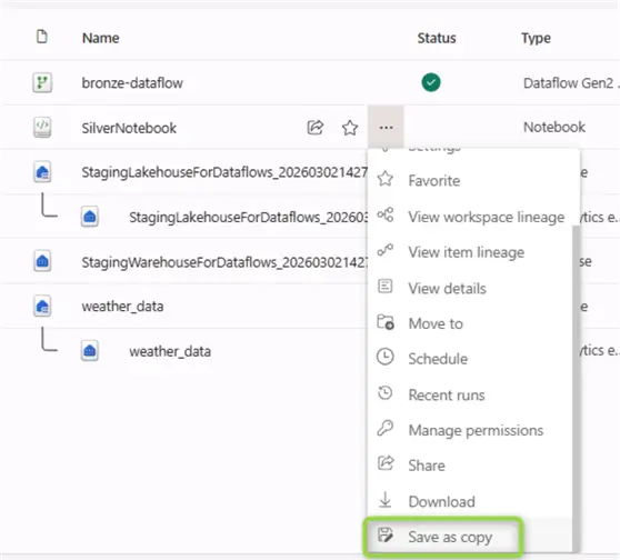
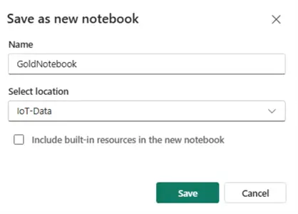
From the workspace home page select the silver notebook and create a copy of it:
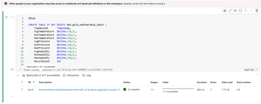
Following the logic we implemented for the silver layer, inside the notebook let us define the target table for the gold layer. Let us say that for the gold table we are interested in reporting the aggregate data for temperature, pressure, and humidity over a 15-min window. Therefore, the schema will be different than the silver layer schema:
--MSSQLTips.com Spark SQL
%%sql

CREATE TABLE IF NOT EXISTS dbo.gold_weatherdata_15min (
    TimeBucket      Timestamp,
    AvgTemperature  DECIMAL(10,2),
    MinTemperature  DECIMAL(10,2),
    MaxTemperature  DECIMAL(10,2),
    AvgPressure     DECIMAL(10,2),
    MinPressure     DECIMAL(10,2),
    MaxPressure     DECIMAL(10,2),
    AvgHumidity     DECIMAL(10,2),
    MinHumidity     DECIMAL(10,2),
    MaxHumidity     DECIMAL(10,2),
    RecordCount     INT
)
Now in the gold layer we must account for several additional points:
- The latest record
- The current time bucket or 15-min aggregation window
Therefore, creating new records or updating in place is now more complex. We will need three queries to combine in our statement:
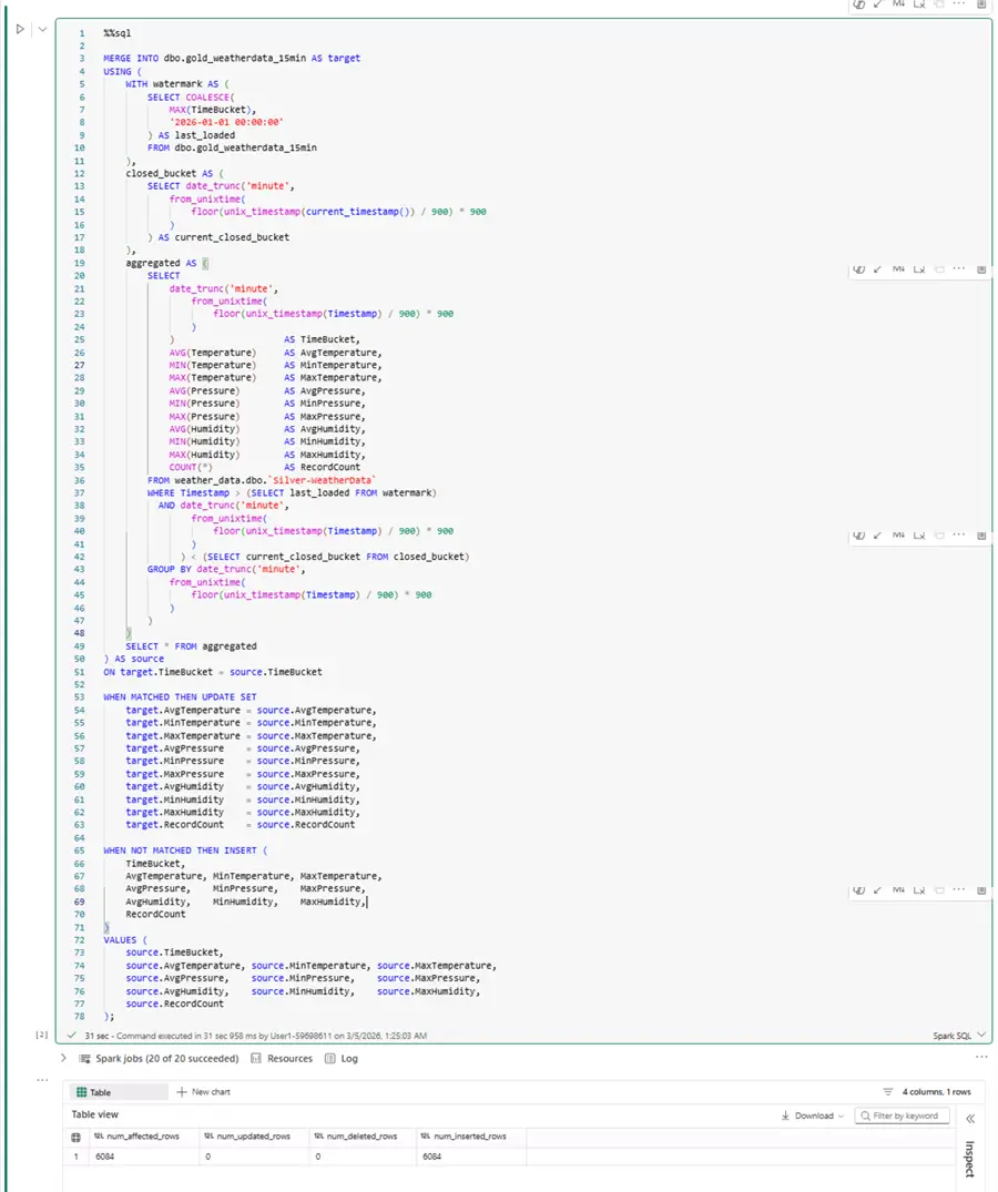
--MSSQLTips.com Spark SQL
%%sql

MERGE INTO dbo.gold_weatherdata_15min AS target
USING (
    WITH watermark AS (
        SELECT COALESCE(
            MAX(TimeBucket),
            '2026-01-01 00:00:00'
        ) AS last_loaded
        FROM dbo.gold_weatherdata_15min
    ),
    closed_bucket AS (
        SELECT date_trunc('minute',
            from_unixtime(
                floor(unix_timestamp(current_timestamp()) / 900) * 900
            )
        ) AS current_closed_bucket
    ),
    aggregated AS (
        SELECT
            date_trunc('minute',
                from_unixtime(
                    floor(unix_timestamp(Timestamp) / 900) * 900
                )
            )                    AS TimeBucket,
            AVG(Temperature)     AS AvgTemperature,
            MIN(Temperature)     AS MinTemperature,
            MAX(Temperature)     AS MaxTemperature,
            AVG(Pressure)        AS AvgPressure,
            MIN(Pressure)        AS MinPressure,
            MAX(Pressure)        AS MaxPressure,
            AVG(Humidity)        AS AvgHumidity,
            MIN(Humidity)        AS MinHumidity,
            MAX(Humidity)        AS MaxHumidity,
            COUNT(*)             AS RecordCount
        FROM weather_data.dbo.`Silver-WeatherData`
        WHERE Timestamp > (SELECT last_loaded FROM watermark)
          AND date_trunc('minute',
                from_unixtime(
                    floor(unix_timestamp(Timestamp) / 900) * 900
                )
              ) < (SELECT current_closed_bucket FROM closed_bucket)
        GROUP BY date_trunc('minute',
            from_unixtime(
                floor(unix_timestamp(Timestamp) / 900) * 900
            )
        )
    )
    SELECT * FROM aggregated
) AS source
ON target.TimeBucket = source.TimeBucket

WHEN MATCHED THEN UPDATE SET
    target.AvgTemperature = source.AvgTemperature,
    target.MinTemperature = source.MinTemperature,
    target.MaxTemperature = source.MaxTemperature,
    target.AvgPressure    = source.AvgPressure,
    target.MinPressure    = source.MinPressure,
    target.MaxPressure    = source.MaxPressure,
    target.AvgHumidity    = source.AvgHumidity,
    target.MinHumidity    = source.MinHumidity,
    target.MaxHumidity    = source.MaxHumidity,
    target.RecordCount    = source.RecordCount

WHEN NOT MATCHED THEN INSERT (
    TimeBucket,
    AvgTemperature, MinTemperature, MaxTemperature,
    AvgPressure,    MinPressure,    MaxPressure,
    AvgHumidity,    MinHumidity,    MaxHumidity,
    RecordCount
)
VALUES (
    source.TimeBucket,
    source.AvgTemperature, source.MinTemperature, source.MaxTemperature,
    source.AvgPressure,    source.MinPressure,    source.MaxPressure,
    source.AvgHumidity,    source.MinHumidity,    source.MaxHumidity,
    source.RecordCount
);
This query has three common table expressions (CTEs):
- watermark: takes the latest timestamp present in the silver lakehouse table.
- closed_bucket: calculates the current bucket with the system function
current_timestamp(). We will use this value to ensure that we do not write to an open 15-min bucket. - aggregated: the core logic for grouping and aggregating the data. To understand the query, which is nothing more than the regular MERGE type of statement, it is important to understand the grouping:
- The first step
unix_timestamp(Timestamp)converts the Timestamp column into a Unix timestamp representing the number of seconds since Jan 1, 1970, e.g., 2024-01-15 09:23:47 becomes 1705311827 - The second step
floor(.../ 900) * 900takes the value for the nearest fifteen-minute boundary (900 = 60 seconds × 15 minutes). Multiplying back by 900 gives the Unix timestamp of that interval’s start. - The third step
from_unixtime(...)converts the fifteen-minute rounded Unix timestamp back into a human-readable datetime string, e.g., 1705311000 becomes “2024-01-15 09:15:00” - The final fourth step
date_trunc('minute', ...)truncates the result to minute precision, stripping any sub-minute noise. This is mostly a safety step to ensure data quality.
- The first step
All three CTEs are a vital part of the MERGE statement which takes care to update existing data (if necessary) or to create new records. Here is how the statements look in practice, together with their first run results:
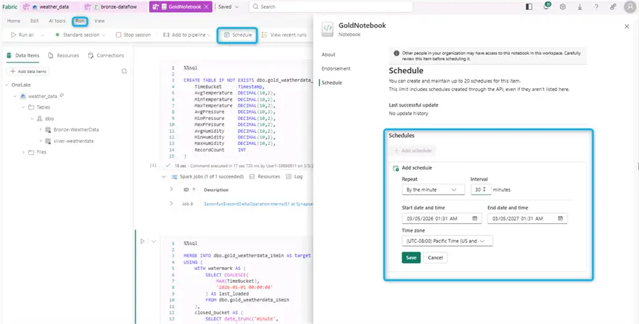
Schedule gold layer ingestion
Like the silver layer ETL notebook, we can create a schedule for the gold transformation:
At this point all layers have been created, together with logic for adding data to each one of them.
Examine gold layer data
Finally, let us do a quick sanity check of the gold layer data:
--MSSQLTips.com Spark SQL
%%sql

SELECT TimeBucket
       , AvgTemperature
       , MinTemperature
       , MaxTemperature
       , AvgPressure
       , AvgHumidity
       , RecordCount
FROM dbo.gold_weatherdata_15min
ORDER BY TimeBucket DESC
LIMIT 10;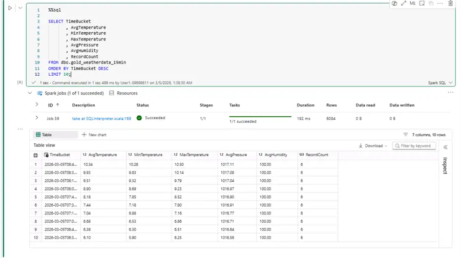
Expectedly, we see a consistent record count of six across all rows. Remember, we had data arriving every 145 seconds originally, so (15 minutes * 60) / 145 ≈ 6. Therefore, every time bucket of 15 minutes should contain six records. As a result, we have cleanly aggregated data ready for the final reporting layer.
Concluding thoughts
Using MS Fabric lakehouse, dataflow gen2, notebooks with Spark SQL we created a medallion architecture for our IoT weather data. Currently the following three delta tables exist:
- Bronze: raw staging data.
- Silver: cleaned, filtered highly granular data.
- Gold: cleaned, filtered, and aggregated data ready for reporting.
The three layers are built on top of each other to provide high quality validated data. The ETL jobs for each layer are decoupled and responsible for the respective stage only; every next stage just needs to use the correct schema, table, and column names.
Next Steps
- Getting Started with Microsoft Fabric
- Microsoft Fabric FAQ
- Microsoft Fabric Architecture FAQ
- Design Data Warehouse with Medallion Architecture in Microsoft Fabric
- Microsoft Fabric vs Power BI
- Data Lake Medallion Architecture to Maintain Data Integrity

Hristo Hristov is a seasoned data professional with 10+ years of experience spanning the intersection of data engineering and smart manufacturing solutions. Since 2017, he has specialized in implementing advanced analytics solutions for bridging the IT/OT gap.
A technical writer with over 80 published articles on data and AI technologies, Python development, and cloud solutions. Passionate about transforming complex data into business value through innovative applications of Azure Data Platform, Python, IoT solutions, databases, and other cloud technologies.
Currently applying Industry 4.0 best practices, focusing on IoT connectivity, and implementing data and AI systems in manufacturing. Hristo holds a degree in Data Science and several Microsoft certifications covering SQL Server, Power BI, and related technologies.
- MSSQLTips Awards
- Achiever Award (75+ tips) – 2026
- Rookie of the Year – 2021
- Author Contender – 2022/2023/2024/2025