Problem
Having worked with traditional RDBMS-based data warehouses for 15 years, I am now faced with a new challenge. Deliver faster, more efficient data streaming capability and integrate it with other Data Lake sources like Dynamics 365 and Microsoft Dataverse database for Power Apps. All this has a very time-restricted delivery.
Solution
This tip provides an example of data lake architecture designed for a sub 100GB data lake solution with SCD1. The Data Lake will have no history, i.e., it will overwrite every time from the source system, which means that the source systems preserve history. The tip will explain how to take general principles of Medallion architecture for the design of Data Lakes and apply it to specific customer cases and how to maintain foreign key relationships between files in a Data Lake.
What is Medallion Architecture in Data Lake?
In short, Medallion architecture requires splitting the Data Lake into three main areas: Bronze, Silver, and Gold. In addition to the three layers, a fourth area called the Landing Zone is needed. These areas are shown in the image below.

Figure 1: Medallion Architecture with 4 Layers
You can find more details on medallion architecture in this tip: Designing a Data Lake Management and Security Strategy.
Why Python with PySpark vs. SQL?
I love SQL; it is structured and treats my data as a set. I do not need to worry about every record or row in my tables. Although, when you need to look at individual records in a given data set, it becomes cumbersome. Moving files around with SQL is hard. And the SQL feature I personally miss is the ability to create or modify classes and other aspects of OOP programming. On the other hand, Python is an OOP language; it can easily manipulate data/files via DataFrame. In Python, you can write and share your functions between notebooks. Python allows developers to perform the same operations in various ways; this is almost the opposite of SQL. When you start with Python, you quickly realize that you must follow self-imposed coding guidelines to maintain structure and coherency in the code. Luckily, python.org has a Python style guide, the PEP8, to use as a base. Furthermore, by using Python, you open up a whole new world of libraries to use for your Data Lake project. You can use Pandas, but I recommend sticking with PySpark as it separates compute from storage and allows for multi-node parallel processing of your DataFrame.
Azure Synapse Analytics vs. Databricks
To manage and run PySpark notebooks, you can employ one of the two popular modern data warehouse platforms. Microsoft offers Azure Synapse Analytics, which is solely available in Azure. Databricks, on the other hand, is a platform-independent offering and can run on Azure, AWS, or Google Cloud Platform. You can find practical examples of implementing Databricks solutions in this tip: Data Transformation and Migration Using Azure Data Factory and Azure Databricks.
For this tip, I will use Azure Synapse Analytics workspace. This Microsoft documentation can help demonstrate how to create a Synapse workspace: Creating a Synapse workspace.
Medallion Layers
Landing Zone
A Landing Zone layer is required to accommodate the differences between source systems and Data Lake. It will contain raw copies of data “as-is” from the source system. Data can be copied here by services like Azure Data Factory/Synapse Analytics or AWS Glue. Some data may be pushed here via the Dataverse link or Dynamics 365 CMD. In short, this area will be strongly determined by source systems and their ability to share data.
I have sample data from the City of New York website where I used data for Q1 and Q2 of 2022 for both Yellow and Green taxi trips and uploaded it to my Azure Storage Account Blob Container called “0-landingzone”:
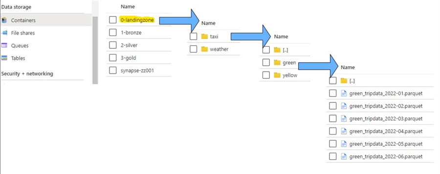
Figure 2: Landing Zone Folder Structure for Taxi Data
Let’s augment taxi data with historical weather data by adding it to our landing zone:
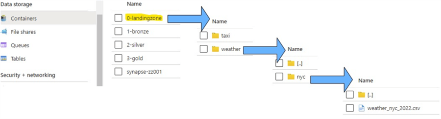
Figure 3: Landing Zone Folder Structure for Weather Data
Bronze Layer. Source systems provide data to the landing zone using their file formats and file hierarchy. The bronze layer standardizes data from the landing zone to your folder and file format. You should consider using the following file formats:
- Parquet – Compressed columnar file format.
- Delta Lake – Versioned parquet files with transaction log and ACID capability.
- AVRO – Row-oriented file format, uses JSON to define data types and protocols and binary format for data.
Each of these file types offers their strengths and weaknesses. Delta Lake is the fastest file format in terms of IO, but requires a cleanup strategy because versioned parquet files are not deleted automatically. AVRO is specifically designed to support row-based access but does not offer the best compression. On the other hand, Parquet is compressed columnar storage that resembles the characteristics of a clustered column store index in a traditional data warehouse. I would choose Parquet, where ACID capability is not required in bronze, and potentially look into Delta format if you must preserve data in bronze at all costs. For this tip, I will use Parquet for the file format storage in bronze.
We will now build a Python notebook that will read out taxi data from the landing zone to PySpark DataFrame, add bronze layer technical fields, and write this DataFrame to conform with the folder and file structure in the bronze layer. I will be using the following Python libraries:
from pyspark.sql.functions import input_file_name
from pyspark.sql.functions import current_timestamp
from pyspark.sql.dataframe import *
Here is the function for reading all Parquet files from any given folder:
def read_files(storage_account, layer, path, file_format):

    """
    This function reads all parquet files associated with one folder
    Parameter storage_account is the storage account name
    Parameter layer is the medallion layer: 0-landingzone, 1-bronze, 2-silver, 3-gold
    Parameter path is the relative folder structure that all parquet files should be read from
    Parameter file_format allows for selection of file formats like CSV or Parquet
    """

    #constructing full path
    full_path = f"abfss://{layer}@{storage_account}.dfs.core.windows.net/{path}/**"
    message = 'reading file from: ' + full_path
    print(message)

    try:
        #reading parquet files to DataFrame
        df = spark.read.option("header",True).format(file_format).load(full_path)
        message = "file successfully read from:" + full_path
        print(message)

    except:
        #failure message
        message = "Failed to read file from:" + full_path
        print(message)

    return  df
I will create a function for adding custom columns to DataFrame and then extend my DataFrame class with this function:
def df_add_columns(df, add_timestamp=False, add_filename=False):

    """
    This function adds bronze layer custom fields
    Parameter add_timestamp determines whether timestamp should be added to dataframe
    Parameter add_filename determines whether landing zone path and filename should be added to dataframe
    """
    #add timestamp column
    if add_timestamp:
        df = df.withColumn(
            "xyz_bronze_timestamp",
            current_timestamp()
        )

    #add full path and filename column
    if add_filename:
        df = df.withColumn(
            "xyz_bronze_filename",
            input_file_name()
        )

    return df

#extending DataFrame class with add_columns function
DataFrame.add_columns = df_add_columns
The last function for the bronze layer transformation will be the write function that executes writes to a Parquet table:
def write_parquet_table(df, storage_account, layer, table_name):

    """
    This function will write dataframe df to storage account as a parquet files
    Parameter table_name defines parquet file name in bronze layer
    """

    #defining full path to in storage account
    full_path = f"abfss://{layer}@{storage_account}.dfs.core.windows.net/{table_name}"
    message = 'writing bronze file: ' + full_path
    print(message)

    try:
        #writing table folder with parquet files in overwrite mode for SCD1
        df.write.mode('overwrite').parquet(path)
        message = 'Table successfully written: ' + full_path
        print(message)

    except:
        #error message
        message = 'Failed to write table: ' + full_path
        print(message)
Now that you have added the libraries and all three functions to your notebook, you can execute the main Python code that will transform the taxi data for both yellow and green company and bring it over to the bronze layer:
storage_account = "change this to your storage account name"

#for loop for each taxi company
for taxi_company_name in ["green","yellow"]:

    #reading taxi data
    layer = "0-landingzone"
    path = f"taxi/{taxi_company_name}"
    df_taxi = read_files(storage_account, layer, path, "parquet")

    #Add timestamp & full filepath and name to dataframe
    df_taxi = df_taxi.add_columns(add_timestamp=True, add_filename=True)

    #write to taxi DataFrame to bronze table
    layer = "1-bronze"
    table_name = f"{taxi_company_name}_taxi"
    write_parquet_table(df_taxi, storage_account, layer, table_name)
Once the code has been executed, you should see the following output. Note: I am executing code in Azure Synapse analytics, and this output may look slightly different in Databricks.
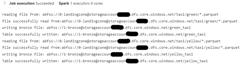
Figure 4: Result of Successful Python Code Execution for Bronze Transformation
This code will add two additional columns: xyz_bronze_timestamp and xyz_bronze_filename, and perform file and folder transformation, as seen in the image below:
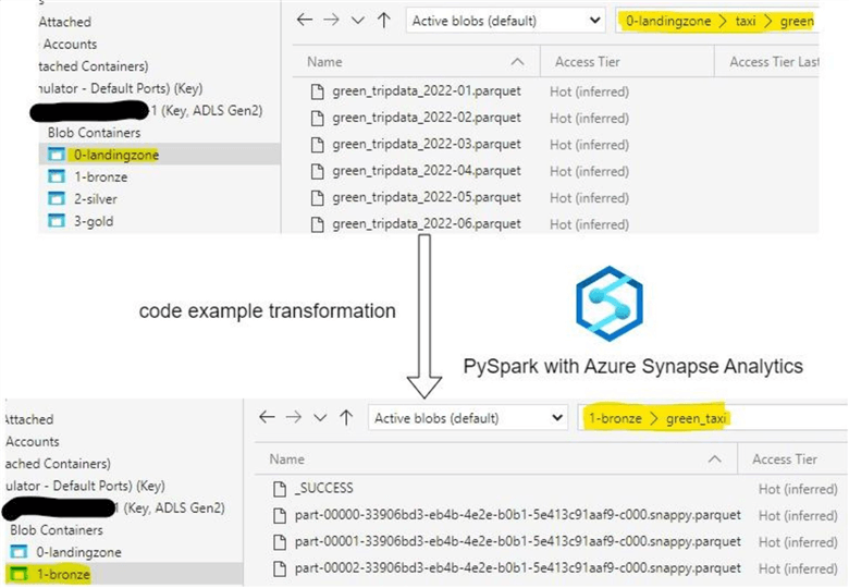
Figure 5: Bronze Layer File Transformation
Timestamp and filename allow for linage control and identifying the origins of data. Yellow and Green taxi data is now stored in the bronze layer in identical file and folder format. Let’s now add our weather data to the bronze layer. This time it will be transformed from a single CSV file to a Parquet table:
storage_account = "change this to your storage account name"

#reading weather data for NYC
layer = "0-landingzone"
path = f"weather/nyc"
df_weather = read_files(storage_account, layer, path, "csv")

#Add timestamp & full filepath and name to dataframe
df_weather = df_weather.add_columns(add_timestamp=True, add_filename=True)

#write weather DataFrame to bronze table
layer = "1-bronze"
table_name = f"nyc_weather"
write_parquet_table(df_weather, storage_account, layer, table_name)
Finally, your file and folder transformations for weather data yield the following structure:
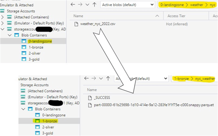
Figure 6: Weather Data Transformation Bronze Layer
Run the print schema command on the weather DataFrame to check that the bronze layer technical fields have been added before they were written to the Parquet table:
df_weather.printSchema()
The last two columns of the DataFrame will be the technical DataFrame columns:
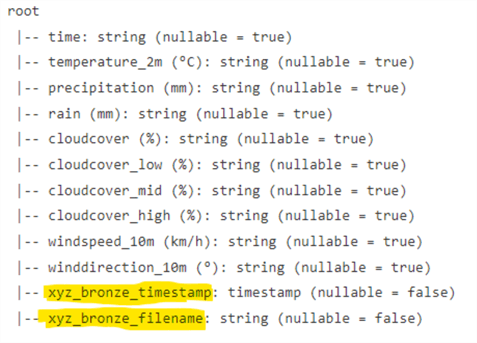
Figure 7: PrintSchema() of Weather Data Showing Timestamp and Filename Columns
Silver Layer. The silver layer resembles the enterprise layer in a traditional data warehouse. The silver layer would normally adhere to the following data design principles:
- Data is normalized.
- Business Keys are unique.
- No duplicate data.
- Data should be augmented with surrogate keys.
- Foreign Key relationships need to be established.
- Data types enforced.
- File format must have ACID capabilities and transaction log, Delta Lake.
In addition, business-critical logic is to be implemented in the silver layer.
Foreign Keys. One key difference between a traditional relational database data warehouse and Spark Data Lake is that you must design your own relationship (foreign keys) management in Spark using Python functions. In this tip, I will be hashing the business key columns and then looking them up against other tables. If hashing fails to return the result, the key value will be “-1” when there is no match; in the lookup table, the key value will be set to “-2”.
To code the example, we will transform the taxi data into two tables: one called companies, containing the taxi company name and corresponding SHA2 hash key in column id_company, and a second table called rides, including reference to the company table and additional information about every ride, like fare, date time, and more:
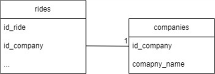
Figure 8: One-to-Many Relationship Between Rides and Companies
I will use the following Python libraries for the silver layer transformation:
from pyspark.sql.types import StructType,StructField, StringType, IntegerType
from pyspark.sql.functions import split, col, concat_ws, lit, sha2, when
from pyspark.sql.dataframe import *
from delta.tables import *
I will reuse the read_files() function from the bronze layer transformation.
The function for calculating the SHA2 hash is given below:
def df_create_sha2_hash(df, columns, hash_column_name="xyz_hash"):
    """
    Uses SHA2 algorithm to hash columns list and creates new column with hash value
    Parameter columns - List of columns that is to be hashed
    Parameter hash_column_name - Name of the column to be hashed. Defaulted to xyz_hash
    """
    null_check = concat_ws("||", *[lit(None) for c in columns])

    #calculating SHA2 for all columns in the list
    df = df.withColumn(hash_column_name, sha2(concat_ws("||", *columns), 256))
    #Setting hash to None if all of the columns is NULL
    df = df.withColumn(hash_column_name, when(col(hash_column_name) == sha2(null_check, 256), lit(None)).otherwise(col(hash_column_name)))
    return df

#extending DataFrame class with add_columns function
DataFrame.create_sha2_hash = df_create_sha2_hash
Here is the Python function for writing the DataFrame to a delta table in SCD1 mode, overwrite:
def write_delta_table(df, table_name, layer="2-silver", logRetentionDuration  = "interval 60 days", deletedFileRetentionDuration  = "interval 15 days"):

    """
    This function writes dataframe to delta table
    Parameter df is the dataframe to be written
    Parameter table_name defines the delta table name
    Parameter layer is either 2-silver or 3-gold
    Parameter logRetentionDuration defines duration for log history of delta table
    Parameter deletedFileRetentionDuration defines retention period before delta table files are to be deleted physically
    """

    #define your storage account and table path
    storage_account = "storageaccountzz001"
    path = f"abfss://{layer}@{storage_account}.dfs.core.windows.net/{table_name}"

    #initiating message
    message = f"writing silver file: {path}"
    print(message)

    try:
        #mode is set to overwrite for SCD1
        df.write.format("delta").mode("overwrite").option("overwriteSchema", "true").save(path)

        #setting delta table log retention duration & deletesFileRetentionDuration
        deltaTable = DeltaTable.forPath(spark, path)
        deltaTable.logRetentionDuration  = "interval 60 days"
        deltaTable.deletedFileRetentionDuration  = "interval 15 days"

        #succsess message
        message = f"file successfully written to: {path}"
        print(message)

    except:
        #failure message
        message = f"failed to write file to: {path}"
        print(message)

Lookup function for looking up id column between two DataFrames with one-to-many relationship:

def df_lookup(df, df_lookup, lookup_column):

    """
    This function will lookup id column in dataframe against dataframe df_lookup
    Function is intended for one-to-many relationship between df and df_lookup

    Parameter df_lookup is the lookup dataframe
    Parameter lookup_column is the id column to lookup
    """

    #filtering only the lookup column and adding second identical column with prefix xyz_
    df_lookup = df_lookup.select(col(lookup_column))
    temp_lookup_column_name = f"xyz_{lookup_column}"
    df_lookup = df_lookup.withColumn(temp_lookup_column_name, col(lookup_column))

    #joining on lookup column
    df = df.join(df_lookup, lookup_column, "left")

    #setting id column value to -1 where value is Unknown/DBNull and -2 where value is NA/NOT FOUND
    df = df.withColumn(lookup_column, when(col(lookup_column).isNull(), lit("-1"))
                                     .when(col(temp_lookup_column_name).isNull(), lit("-2"))
                                     .otherwise(col(lookup_column))
                                     )

    #dropping the temporary column
    df = df.drop(temp_lookup_column_name)

    return df

DataFrame.lookup = df_lookup
The code below will create and populate a static table called companies with the company name and corresponding SHA2-256 hash:
#data
company_data = [
    ("c685a2c9bab235ccdd2ab0ea92281a521c8aaf37895493d080070ea00fc7f5d7", "yellow"),
    ("ba4788b226aa8dc2e6dc74248bb9f618cfa8c959e0c26c147be48f6839a0b088", "green"),
    ("-1", "UNKNOWN or DbNull"),
    ("-2", "N/A or NOT FOUND")
]

#schema definition
company_schema = StructType([     StructField("id_company",StringType(),True),     StructField("company_name",StringType(),True),   ])

#create dataframe
df_company = spark.createDataFrame(data=company_data, schema=company_schema)

#srite dataframe to silver layer as delta table
write_delta_table(df_company, "companies", layer="2-silver")

display(df_company)
Company DataFrame should display the following result:
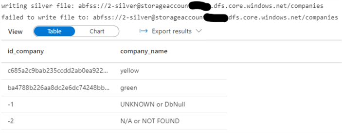
Figure 9: Silver Layer Company DataFrame
The last step for the silver layer will be to read both the yellow and green taxi data from bronze, union the data into one DataFrame, enforce data types, and perform a lookup of id_company against the company table to find if we have any mismatching hash keys:
storage_account = "Change this to your storage account name"

#reading yellow taxi data
df_yellow_taxi = read_files(storage_account, "1-bronze", "yellow_taxi", "parquet").selectExpr(
    "VendorID",
    "tpep_pickup_datetime as pickup_datetime",
    "xyz_bronze_filename",
    "trip_distance",
    "fare_amount"
)

#reading green taxi data
df_green_taxi = read_files(storage_account, "1-bronze", "green_taxi", "parquet").selectExpr(
    "VendorID",
    "lpep_pickup_datetime as pickup_datetime",
    "xyz_bronze_filename",
    "trip_distance",
    "fare_amount"
)

#union green taxi data with yellow
df_taxi = df_yellow_taxi.union(df_green_taxi)

#getting taxi company name from file path
df_taxi = df_taxi.withColumn("company_name", split(col("xyz_bronze_filename"), "/").getItem(4))

#creating hash id for business key
df_taxi = df_taxi.create_sha2_hash(["VendorID", "pickup_datetime"], "id_ride")

#creating hash id for company key
df_taxi = df_taxi.create_sha2_hash(["company_name"], "id_company")

#lookup against company write_delta_table
df_taxi = df_taxi.lookup(df_company,"id_company")

#writing data frame to delta table in silver
write_delta_table(df_taxi, "rides", layer="2-silver")

df_taxi.printSchema()
After the Python code execution, the rides table will have the following metadata:
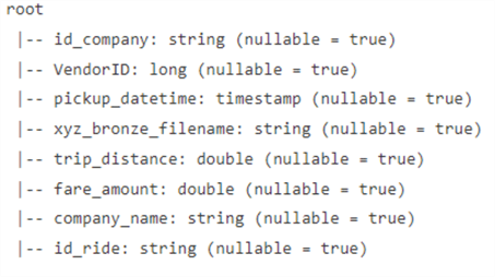
Figure 10: Rides Delta Table Metadata
The rides delta table, id_company column, will be set to “-1”, where the column hash calculation has resulted in an unknown value, and “-2”, where there is no match between the rides and companies tables. Notice that we only took a subset of columns from bronze to silver. You should only take columns that you intend to use to the silver layer to avoid complexity run-away that may result in a data swamp. The more fields you bring over from bronze to silver, the harder it becomes to maintain a consistent and coherent model that is well-normalized.
Gold Layer. The gold layer is the presentation layer, where silver tables get transformed and rearranged to Kimball star architecture to be later consumed by report building applications like Power-BI or Tableau. This layer should be deformalized by removing some of the complexity of the silver layer. You may want to use the same silver layer data in different perspectives called data marts. You would typically design one data mart per end consumer group to make the data friendly and easy to consume by other professions than data specialists.
As an example, we will use our taxi rides and company table and perform aggregation transformation by aggregating all rides to the lowest granularity of one day and then present these tables in the gold layer with new names, fact_ride and dim_company:
storage_account = "Yours storage account name"

#reading rides data from silver layer
df_rides = read_delta_table(storage_account, "2-silver", "rides")

#getting date part of datetime column
df_rides = df_rides.withColumn('id_date', to_date(col('pickup_datetime')))

#aggregate tides data by date
df_fact_ride = df_rides.groupBy("id_date")         .agg(first("id_ride").alias("id_ride"),              first("id_company").alias("id_company"),              count("id_ride").alias("nr_of_rides"),              sum("trip_distance").alias("sum_trip_distance"),              sum("fare_amount").alias("sum_fare_amount"))

#writing data frame to delta table in gold
write_delta_table(df_fact_ride, "fact_ride", layer="3-gold")

df_fact_ride.printSchema()
The code output should look like this:
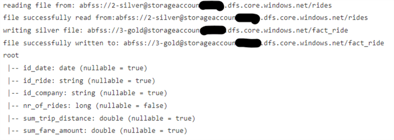
Figure 11: Fact_ride Transformation from Silver to Gold
Furthermore, you can bring the company table from silver to gold layer table dim_company and generate dim_date using either Python code examples or SQL code from this tip: Creating a date dimension or calendar table in SQL Server.
Here is the potential data mart star architecture for the gold layer using the taxi data:
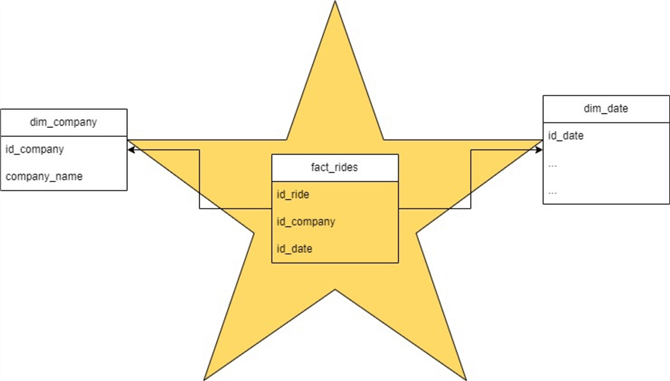
Figure 12: Gold Layer Ride Star Schema
Delta Lake Files Maintenance by VACUUM. As I previously mentioned, Delta tables require additional maintenance. Delta file format transaction log will remove old Parquet files from its manifest after a specified time period has elapsed called logRetentionDuration. Parquet files removed from the log manifest will only be marked for deletion once another period called deletedFileRetentionDuration is overdue. The deletion itself is performed using Spark SQL only command called VACUUM. An example is illustrated below:
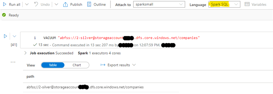
Figure 13: Example of VACUUM Command with Azure Synapse Analytics PySpark
Summary
Whether you are entirely new to data engineering, transferring from traditional BI to the new world of Data Lake, or just mastering your skills, Medallion architecture is an excellent tool for modern Data Lake. It allows source system abstraction using the bronze layer and the ability to build complex enterprise models in silver. You will keep your data consumers in the gold layer to abstract complexity and internal logic.
Next Steps
- SCD2 with Databricks
- Exploring the Capabilities of Azure Synapse Spark External Tables
- Writing Databricks Notebook Code for Apache Spark Lakehouse ELT Jobs

Semjon Terehhov is an MCSE in Data Management and Analytics, Data consultant & Partner at Cloudberries Norway. He has a master’s degree from the University of Oxford. For the past 10 years, I have worked as a DBA, BI Developer, and DevOps starting with SQL Server 2005. I have worked from the hardware up all the way through to the stack to the front end programming to design data solutions for end-users needs.


This is a great article, thanks a lot!
Hi, where do you download the nyc weather file 2022 ?
Such a lovely and helpful article thanks very much