Using T-SQL to Assess Goodness of Fit to an Exponential Distribution

By: Rick Dobson | Comments | Related: > TSQL

Problem

Please provide a framework with SQL code for assessing if a set of data values conform to an exponential distribution. Explain the guidelines for assessing goodness of fit for a set of data values to an exponential distribution. Provide several worked examples of the SQL code using different data values to confirm the operation and robustness of the solution framework.

Solution

One classic data science project type is assessing the goodness of fit for a set of data values to a distribution; see here and here for other data science project types and how to do data science with SQL. The reasons for wanting to know if data conform to a distribution mostly depend on the distribution. An exponential distribution can be useful for modeling the distribution of times to failure for manufactured items, interarrival times of phone calls to a call center, and times between Geiger clicks for radioactive materials.

You can assess with the Chi Square distribution the goodness of fit of observed values to expected values, such as those from an exponential distribution. This tip focuses on how to code and interpret Chi Square test results for goodness-of-fit to an exponential distribution. In this tip, a framework is presented and evaluated for three sample sets of data to assess goodness-of-fit to an exponential distribution. This same framework also applies generally to other kinds of distributions; subsequent tips will demonstrate this.

The Chi Square goodness-of-fit test is different than other popular kinds of statistical tests for at least two reasons.

First, the Chi Square goodness-of-fit test processes frequencies or counts for a set of bins. In contrast, both a t-test and an ANOVA test process means for one or more groups of data.
Second, you confirm with the Chi Square goodness-of-fit test an a priori assumption about the source distribution for a set of data values by accepting the the null hypothesis of no difference between the observed and expected frequencies, but with other statistical tests you commonly reject the null hypothesis to confirm an a priori assumption.
- With a Chi Square test, you accept the goodness of a fit when you can't reject the null hypothesis that the observed frequencies conform to the expected frequencies.
- With other kinds of statistical tests, you can assert that the means are different when you can reject the null hypothesis of no differences between the means.

Introduction to Goodness-of-fit Chi Square test

The Chi Square goodness-of-fit test compares observed frequencies by bin to expected frequencies by bin. Each bin is defined by bottom and top values. The frequencies are counts of values between bottom and top bin boundaries. The expected frequencies come from assumptions about the distribution and the expected count of values between the top and bottom bin boundaries per bin. If there is no statistically significant difference between observed and expected frequencies across the full set of bins, then the observed frequencies are confirmed not to differ significantly from the distribution for expected frequencies - that is, the observed values are a good fit to the expected values.

The following expression is for a computed Chi Square value. Values of i extend over the bins used to compare observed values to expected values. Each bin is defined by a bottom value and a top value. The comparisons are performed over a total of k bins for i values that start at 1 and extend through k. SQL developers can think of the source data for the computation of a Chi Square value as a table with three columns: the first column is for the bin identifier (values of i), the second column is for the count of observed values between the bottom and top values for each bin (O_i), and the third column is for the count of the expected values between the bottom and top values for each bin (E_i).

Sum ((O_i - E_i)²/E_i)

You can interpret the statistical significance of a computed Chi Square value by comparing it to a critical Chi Square value. When the computed Chi Square value exceeds or equals a critical Chi Square value, then the null hypothesis of no difference between the observed and expected frequencies is rejected. Otherwise, the observed frequencies are accepted as being derived from a distribution used to calculate the expected values. The total counts of observed and expected values should be identical.

As with other kinds of statistical tests, the Chi Square goodness-of-fit test has both degrees of freedom and probability levels for interpreting the level of statistical significance associated with a computed test value. These two parameters determine the critical Chi Square value for determining whether a computed Chi Square value is statistically significant. If you are evaluating a computed Chi Square value for statistical significance at multiple probability levels, then you should compare the computed Chi Square value to multiple critical Chi Square values. The Excel CHISQ.INV.RT built-in function generates critical Chi Square values for specified degrees of freedom and designated probability levels.

The following screen excerpt is from an Excel workbook file with critical Chi Square values. The cursor rests in cell B2. This cell displays the critical Chi Square value (3.841459) for one degrees of freedom at the .05 probability level. The formula bar displays the expression for deriving a critical value. The workbook displays critical values for three commonly reported probability levels - namely: .05, .01, and .001; these values populate, respectively, cells B1, C1, and D1. The full workbook contains critical Chi Square values at each of these probability levels for degrees of freedom from 1 through 120.

You can import the workbook values into a SQL Server table to facilitate the automatic lookup of a statistical significance of a computed Chi Square value at a probability level. The workbook file name is Chi Square Critical Values at 05 01 001.xls; this file is among those in the download for this tip (see the Next Steps section). This file is in a 97-2003 Excel file format to facilitate its import to a SQL Server table with the SQL Server Import/Export wizard.

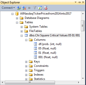
For the purposes of this tip, the Chi Square Critical Values at 05 01 001.xls file is imported to SQL Server as a table named Chi Square Critical Values 05 01 001. The following screen shot displays the design of the table in Object Explorer. The df/prob. column holds degrees of freedom values. Therefore, it has an int data type. The .05, .01, and .001 are in the 05, 01, and 001 columns. These columns have a float data type to accommodate the maximum number of digits returned by the Excel CHISQ.INV.RT built-in function, which also returns a float data type value in Excel.

The next screen shot shows the table in the AllNasdaqTickerPricesfrom2014into2017 database in Object Explorer. However, you can import the table in any database of your choice.

The following screen shot shows a set of excerpted values from the Chi Square Critical Values at 05 01 001.xls file displayed within the Chi Square Critical Values 05 01 001 table in the AllNasdaqTickerPricesfrom2014into2017 database. The SQL Server table reveals more digits than appear with default formatting from within the Excel workbook file. Computed Chi Square values are compared with critical Chi Square values up to the maximum number of digits available. The 05, 01, and 001 columns hold critical Chi Square values for the .05, .01, and .001 values.

The degrees of freedom column identify which set of critical values are used for evaluating the significance level of a computed Chi Square value. The degrees of freedom for the critical Chi Square value is n - 1 - r. The value of n denotes the number of bins. The value of r denotes the number of parameters for the distribution function to compute the expected frequencies. The r value is 1, which is for a parameter named lamda, when using an exponential distribution to compute expected frequencies.

When you are calculating expected frequencies for an exponential distribution or any distribution with continuous values based on the solution framework described, you need a cumulative probability density function (often called a cumulative density function). One common approach adopted for this tip is to find a set of bins with equal proportions over the cumulative density function. For example, if you are going to use eight bins, then each bin should contain one-eighth of the cumulative density function range or .125. If you were using ten bins, then each bin should contain one-tenth of the cumulative density function - namely, .1. There is no fixed number of bins to use for a goodness of fit test.

The Excel Master Series blog denotes three criteria that should be met for a valid Chi Square goodness-of-fit test. These criteria are as follows.

The number of bins should be greater than or equal to five.
The minimum expected frequency for any bin should be at least one.
The average number of expected values across bins should be at least five.

According to Wikipedia, the probability density function (pdf) for an exponential distribution is specified by the following expression. The value for lambda is the inverse of the mean of the observed values.

Wikipedia defines in the same article the cumulative density function (cdf) for an exponential distribution with the following expression. The pdf and cdf are two alternative ways of characterizing probabilities for random variable values, but for some applications, such as the solution framework presented in this tip, the cdf can be easier to use.

The cumulative density function values are defined over a range from zero through one. Therefore, it is straightforward to calculate a set of bottom and top values for any number of bins each with the same proportion. The framework presented in the next section illustrates how to accomplish this with SQL code.

The first SQL Chi Square goodness-of-fit framework example

The framework for computing a Chi Square goodness-of-fit test for a set of values to an exponential function follows the computational guidelines originally presented by professor Kendall E. Nygard from North Dakota State University. This web page presents the guidelines from his statistics lecture note for the computer science curriculum. This tip demonstrates a SQL-based approach to implementing the computational guidelines.

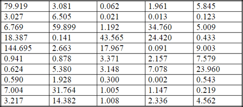
The following display shows the basic data for professor Nygard's Chi Square goodness-of-fit example. The data are for the lifetime in days of microprocessors running at 1.5 times nominal voltage. The key points are that we have a collection of values. The number of values in this example is fifty. In general, you should have enough values to reliably estimate the source distribution for the values. In this tip, you can see that different analysts are using samples as small as thirty values. Recall also that the Excel Master Series blog provides criteria for when it is appropriate to apply a Chi Square goodness-of-fit test.

The next display shows the output from the next-to-last step in professor Nygard's example. This output consists of the bin boundaries, the calculated observed frequencies by bin (O_i), the calculated expected frequencies by bin (E_i), and the last set of column values represent the component from individual bins for the computed Chi Square value. As you can see, there are eight bins.

The bin boundaries appear in the INTERVAL column.
- Within each cell, the first number is for the bottom boundary, and the second number is for the top boundary.
  - As the probability density function expression for an exponential distribution indicates, the initial bottom boundary value is zero; see the expression towards the end of the preceding section.
  - The top boundary value on a theoretical basis for the last bin is infinity (symbol of an eight on its side). For any particular goodness-of-fit test with a sample of data, the top value can be any value which is larger than any other observed value. For example, the top boundary value can be the maximum observed value plus one.
- The intermediate boundary values are computed so that they segment the cumulative density function (cdf) range of zero through one into eight bins with an equal share of the cdf range.
  - More generally, you can choose any number of bins greater than or equal to five.
  - You should not specify so many bins that the average number of expected counts per bin drops below five or that the expected count for any bin declines below one.
In order for an observed value to count among those for a bin, it must be greater than or equal to the bottom boundary value and less the top boundary value.
Because the bins represent equal segments of the cumulative density function range and the decay function is the same at any point along the pdf, each expected frequency is 6.25. The sum of the eight expected frequencies is fifty for this sample data, which is the same as the total number of values for the sample data.
Professor Nygard's lecture note includes expressions for calculating bin boundaries as well as expected frequencies. Observed frequencies derive from comparing the observed values to the bottom and top boundaries of each bin to find to which bin the observation should count.
The last column in the following table contains components for the computed Chi Square value. There is one component for each bin. The sum of the component values across bins is the computed Chi Square for the goodness of fit of the observed values relative to the expected values.

As you can see, the computed Chi Square component values can vary from one bin to the next. Also, the component for the first bin is especially large (26.01) in the sample data set. This single component causes the computed Chi Square value to exceed the critical Chi Square value for a probability level of .001. Professor Nygard reports the sum of the components across all bins as 39.6.

In order to determine the .05, .01, and .001 critical Chi Square values for the sample data we must look up the three critical values in a table of critical values, such as the Chi Square Critical Values 05 01 001 table in the AllNasdaqTickerPricesfrom2014into2017 database. With eight bins, the degrees of freedom for an exponential distribution is 6; the expression for computing the degrees of freedom is given in the "Introduction to Goodness-of-fit Chi Square test" section. The preceding excerpt from the Chi Square Critical Values 05 01 001 table displays critical values of 12.591587243744, 16.8118938297709, and 22.4577444848253 for the .05, .01. and .001 probability levels at six degrees of freedom. Because the computed Chi Square value exceeds even the .001 level, we can reject the null hypothesis that the observed values are distributed as an exponential distribution.

The SQL code for processing the sample data presented and processed manually by professor Nygard has five major segments. These are sequentially presented and discussed in this tip, but the segments run from a single script containing all five segments.

Before the first step, there is a use statement designating a default database. This is the database into which you import the critical Chi Square values table (Chi Square Critical Values 05 01 001). Recall that this table is based on an imported version of the Chi Square Critical Values at 05 01 001.xls Excel workbook file, which is available as a download from this tip (see the Next Steps section).

The first script segment reads the sample data to be evaluated for goodness of fit to an exponential distribution into a table. The table has a name of #temp. A bulk insert statement populates the table based on a text file. The values in the #temp table have a float data type.

use AllNasdaqTickerPricesfrom2014into2017
go

-- example is from this url (http://www.cs.ndsu.nodak.edu/~nygard/csci418/lecture_slides/lec3_stat2.htm)
-- step 1: import duration data for estimating 
-- exponentially distributed bin counts

begin try
drop table #temp
end try
begin catch
print '#temp not available to drop'
end catch
go

-- Create #temp file for 'C:\for_statistics\processor_lifetime_days.txt'
CREATE TABLE #temp(
 durations float 
)

-- Import text file
BULK INSERT #temp
from 'C:\for_statistics\processor_lifetime_days.txt'
with (firstrow = 2)

In the code excerpt above, the file with the source data has the name processor_lifetime_days.txt. This file resides in the c:\for_statistics path. For this type of example, the data file contains a single column of values. The following pair of screen shots shows the first six rows of a Notepad++ session and the last five rows of a Notepad++ session with observed values. The first display includes six rows -- a column header (Durations) as well as the first five values from the first row of source data presented by professor Nygard. Because the file starts with a label value (Durations), the SQL code for reading the file starts with the second line (firstrow = 2). The last five rows from the source data appear in the second screen shot for the Notepad++ session.

The second step is to estimate the value of lambda for the exponential distribution based on the sample data in the #temp table. This value is simply the inverse of the mean. The select statement in this code segment merely displays the computed values to confirm their value in the output from the script.

-- step 2: compute average duration and rate
-- is the inverse of average and vice versa
select 
 avg(durations) avg_durations
,1/avg(durations) lambda 
from #temp

The third step is to compute the bottom and top boundaries for a set of bins. The bottom and top bin boundary values are stored in the #bin_bottom_top_duration table. The calculation and storing of these boundary values rely on some local variables.

The @total_bins variable is the total number of bins into which you want to group values. Recall that this value must be greater than or equal to five. This goodness-of-fit framework demonstration uses the same value as professor Nygard - namely, eight.
The @bin_number variable is an identifier for sequential bins. The @bin_number value is initialized to one for the first bin. The @bin_number value increases by one for each successive pass through a while loop. Within each pass through the loop, case statements calculate and assign bottom and top boundary values for the current @bin_number identifier.
The @bin_bottom and @bin_top variables hold values for the top and bottom bin values of the current pass through the while loop. These variables are initialized prior to the first pass through the loop. A set statement after a declare statement before the loop assigns the value 1/@bin_total to the @bin_top variable. On each pass through the loop, the @bin_bottom and @bin_top variables are assigned along with the @bin_number variable to column values in a row within the #bin_bottom_top_duration table.

The While Loop has three functions.

It moves successively through bin identifier values from one for the first bin through the last identifier value (@total_bins) for the last bin. On each pass through the loop, it inserts a row into the #bin_bottom_top_duration table.
Within each pass, the loop assigns new values to the @bin_bottom and @bin_top variables. The expressions for these assignments use the SQL log function, which is a mathematical natural log function based on the value of e (approximately equal to 2.71828). The natural log function is used to compute the cumulative density function for the exponential distribution. The first and last cumulative density function values for a bin are multiplied by the mean duration value to compute bottom and top bin boundary values.
After the computation of boundary values for a bin and their insertion into the #bin_bottom_top_duration table, the @bin_number, @bin_bottom, and @bin_top variables are assigned fresh values before the next pass through the loop.

-- step 3: #bin_bottom_top_duration table
-- declare local variables populating

declare 
 @total_bins as tinyint = 8
,@bin_number as tinyint = 1
,@p_bin_bottom as float = 0
,@p_bin_top as float = 0

-- initialize  @p_bin_top
set @p_bin_top = 1.0/cast(@total_bins as float)


-- create fresh copy of #bin_bottom_top_duration
begin try
drop table #bin_bottom_top_duration
end try
begin catch
print '#bin_bottom_top_duration is not available to drop'
end catch

CREATE TABLE #bin_bottom_top_duration(
 bin_number tinyint
,duration_bottom float
,duration_top float
)

-- populate #bin_bottom_top_duration
while @bin_number <= @total_bins
begin

insert #bin_bottom_top_duration 
select 
 @bin_number bin_number
,duration_bottom =
 case
	when @bin_number = 1 then 0.0
	when @bin_number > 1
		then -(select avg(durations) from #temp)*log((1.0 - @p_bin_bottom))
	else null

 end 
,duration_top =
 case
	when @bin_number < @total_bins 
		then -(select avg(durations) from #temp)*log((1.0 - @p_bin_top))
	when @bin_number = @total_bins 
		then (select max(durations) + 1 from #temp) 
	else null
 end 

set @bin_number = @bin_number + 1 
set @p_bin_bottom = @p_bin_top
set @p_bin_top = @p_bin_top + 1.0/cast(@total_bins as float)

end

The code for the fourth excerpt appears below. This code excerpt has two main functions. First, it declares and populates some scalar local variables as well as a table variable named @index_durations. Second, a pair of nested while loops assigns bin identifier values to the original set of duration values. Third, the assigned bin identifier values are counted to populate the #observed_by_bin_counts table with the count of observed values belonging to each bin.

The code is designed to be very general and accommodate any number of observed values as well as any number of bins. The local variables especially accommodate this capability. The table variable has the name @index_duration. This table variable has three columns.

The duration_index column is populated by sequential row number index values order by durations values from the #temp table. These row number values are uniquely associated with each source data value.
The durations column are the original source data values from the #temp table.
The bin_number value offers a storage location for associating each observed value from the #temp table with a bin_number value based on which bins an observed value matches in the #bin_bottom_top_duration table.

The use of a pair of nested while loops is a technique for successively searching for which bin number each durations value from the @index_duration table variable matches in the #bin_bottom_top_duration table.

The outer loop successively progresses through durations values in the @index_duration table variable.
The inner loop compares the current durations value from the @index_duration table variable to bottom and top bin boundary values in the #bin_bottom_top_duration table. When a durations value falls between a bin's bottom and top bin boundary limits, then the bin's identifier number is assigned to the bin_number column in the @index_duration table variable.

The final select statement in the following code block counts the bin_number assignments to durations values in the @index_duration table variable and saves the counts by bin number in the #observed_by_bin_counts table. These counts are one of the two sets of frequencies required for a computed Chi Square value.

-- step 4: create fresh copy of #observed_by_bin_counts
begin try
drop table #observed_by_bin_counts
end try
begin catch
print '#observed_by_bin_counts is not available to drop'
end catch


-- declarations for local variables
-- and population of @index_durations for 
-- assigning bin_number values to declarations
declare 
 @durations_count int = (select count(*) from #temp)
,@durations_index int = 1
,@bin_count tinyint = (select count(*) from #bin_bottom_top_duration)
,@bin_index tinyint = 1

declare @index_durations table (duration_index int, durations float, bin_number tinyint)

insert into @index_durations (duration_index, durations)
select row_number() over (order by durations) durations_index, durations from #temp

-- nested loops through @bin_index <= @bin_count
-- and  @bin_index <= @bin_count
while @durations_index <= @durations_count
begin
	
	-- find the maximum durations_top for a durations value
	-- assign bin_number in @index_durations based on maximum 
	-- durations_top value
	while @bin_index <= @bin_count
	begin
		if (select durations from @index_durations where duration_index = @durations_index) <= 
			(select duration_top from #bin_bottom_top_duration where bin_number = @bin_index)
			begin
				update @index_durations
				set bin_number = @bin_index
				where duration_index = @durations_index
				set @bin_index = 1
				break
			end


		set @bin_index = @bin_index + 1
	end
	set @durations_index = @durations_index + 1

end 


-- populate #observed_by_bin_counts with observed
-- counts from bin_number assignments in @index_durations
select bin_number, count(*) observed_count
into #observed_by_bin_counts
from @index_durations
group by bin_number

The fifth step computes expected counts by bin and then compares these counts with the observed value bin counts via the Sum function expression in the "Introduction to Goodness-of-fit Chi Square test" section. The fifth step also looks up the critical values for probability levels for obtaining the computed Chi Square value. Recall that if the probability level is statistically significant with a value of .05, .01, or .001 levels, then you can reject the null hypothesis that the actual values are distributed as an exponential distribution. However, if the probability level for a computed Chi Square value is not statistically significant at the .05 probability level, then you accept the null hypothesis that the original values are distributed according to an exponential functional. All these operations along with others not mentioned are implemented in the following script segment.

The fourth step computes the observed frequencies by bin number. The fifth step adds the computation of frequencies by bin number for expected values. Recall that this tip's framework for assessing if values are exponentially distributed depends on a set of bins that are of equal width based on the cdf. Therefore, the expected frequency count per bin is a constant value that is equal to one divided by the number of bins. The constant value for an expected frequency in the framework does not necessarily have to be an integer number value. Instead, it can be a decimal number with a fractional component, such as 6.25, which is the expected count value per bin in the data for this example.

Here's how the fifth step in the following code segment operates.

The first code segment outputs the computed Chi Square and the degrees of freedom based on nested queries.
- The innermost query (for_computed_chi_square_by_bin) gathers the observed frequencies and the expected frequencies by bin number.
- An intermediate level query (for_overall_chi_square) computes the Chi Square component for each bin.
- The outermost query computes the sum of the Chi Square components across bins (@computed_chi_square) and degrees of freedom (@df).
The second code segment displays observed and expected counts by bin_number along with duration_bottom and duration_top values.
The third code segment looks up the probability level of rejecting the null hypothesis and displays that probability along with the computed Chi Square value.

-- step 5: compute and store computed Chi Square and degrees of freedom
declare @computed_chi_square float, @df int

select 
 @computed_chi_square = sum(chi_square_by_bin)
,@df = COUNT(*) - 1 - 1 
from
(
-- compute chi square by bin
select 
bin_number
,observed_count
,expected_count
,(POWER((observed_count - expected_count),2)/expected_count) chi_square_by_bin
from
(
-- display observed and expected counts by bin
select distinct 
 #bin_bottom_top_duration.bin_number
,#bin_bottom_top_duration.duration_bottom
,#bin_bottom_top_duration.duration_top
,#observed_by_bin_counts.observed_count
,(select count(*) from #temp) * (1.0/cast(@total_bins as float)) expected_count
from #observed_by_bin_counts
left join #bin_bottom_top_duration
on #observed_by_bin_counts.bin_number = #bin_bottom_top_duration.bin_number
) for_computed_chi_square_by_bin
) for_overall_chi_square



-- display observed and expected counts by bin_number
-- along with duration_bottom and duration_top values
select 
 #bin_bottom_top_duration.*
,#observed_by_bin_counts.observed_count
,(select count(*) from #temp) * (1.0/cast(@total_bins as float)) expected_count 
from #observed_by_bin_counts
left join #bin_bottom_top_duration
on #observed_by_bin_counts.bin_number = #bin_bottom_top_duration.bin_number


-- look up and probability of computed Chi Square
select
@computed_chi_square [computed Chi Square]
,
case
	when @computed_chi_square >= [001] then 'probability <= .001'
	when @computed_chi_square >= [01] then 'probability <= .01'
	when @computed_chi_square >= [05] then 'probability <= .05'
	else 'probability > .05'
end [Chi Square Probability Level]
from [Chi Square Critical Values 05 01 001] where [df/prob.] = @df

The following display shows the output from running the preceding set of scripts. The middle pane especially facilitates the comparison of the output from the script segments with the web-based results in professor Nygard's lecture note. The comparison of the code's output to professor Nygard's lecture note confirm the valid operation of the SQL code and the ability of the code to assess the goodness of fit for source values to an exponential distribution.

Note that the duration_bottom and duration_top values from the output match to within one place after the decimal point the interval boundaries from the lecture note. The code's output is more accurate to more places after the decimal because it does not perform any rounding of values used as input for the interval boundary expressions.
There is one exception pertaining to the match of bin boundaries. This is for the duration top value for the last bin. The code's output shows a precise duration top value that is one larger than the maximum source data value. Professor Nygard designates a top interval value for the last bin of infinity, which is not a precise numerical value. However, the top duration for the last bin is larger than any value in the source data. For any given set of source data, the code automatically computes the duration top value for the last bin as the maximum source value plus one. This re-computed value functions as infinity for any particular sample of values.
The observed frequencies in the code's output and the professor's web-based results match exactly for each bin. Also, the expected value is 6.25 in both the code's output and the published lecture note.
Finally, the computed Chi Square is 39.6 in both cases. The code's output indicates that the probability is significant at or beyond the .001 level. Professor Nygard reports the results as significant with a level of .05. The computed value from the SQL-based framework includes the result reported by professor Nygard.

The SQL Chi Square goodness-of-fit framework with interarrival times

One test of the robustness of the goodness-of-fit solution framework and SQL code is to test it on some fresh data. This section refers to an excerpt from a PowerPoint package prepared by Professor Winton from the University of North Florida. The overall PowerPoint package examines several different models for assessing the goodness of fit of source data to several different distributions, including a uniform, normal, and an exponential distribution. It is also relevant to point out that professor Winton examines four different statistical models for assessing goodness of fit (Chi Square, Kolmogorov-Smirnov, Anderson-Darling, and G-Test).

The final two slides present data and goodness-of-fit results for an exponential distribution (see below). There are a couple of key points to note.

The source data values in the first slide image are interarrival times versus the lifetime survival data from the prior example.
There are only thirty source data values versus fifty source data values in the prior example.
It is also noteworthy that professor Winton does not in this example use a Chi Square test to assess goodness of fit. Instead, he uses the Kolmogorov-Smirnov test.

The next screen shot shows the untransformed interarrival times from the first slide in a Notepad++ session. The thirty values in this screen shot from the Notepad++ session are in the same order as the untransformed values from the first slide above. This display differs slightly from the initial example in the prior section in that there is no column header for the interarrival times. As a result, a slight modification is required in the code for reading the source data.

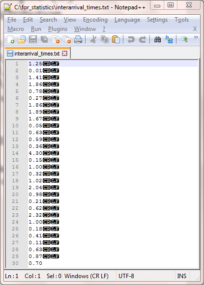
Here's the new code for reading the interarrival times in Professor Winton's example. Notice that the bulk insert statement has changed slightly from the prior section. The sample data from the prior example started with the second line from the data file, but this example starts with the first line. If a code modification were not made, then the data value on the first line would be omitted, and there would be twenty-nine instead of thirty values in the #temp table.

use AllNasdaqTickerPricesfrom2014into2017
go

-- example is from this url 
-- (https://www.unf.edu/~cwinton/html/cop4300/s09/class.notes/c3-GoodnessofFitTests.pdf)
-- import duration data for estimating 
-- exponentially distributed bin counts

begin try
drop table #temp
end try
begin catch
print '#temp not available to drop'
end catch
go

-- Create #temp file for 'C:\for_statistics\interarrival_times.txt'
CREATE TABLE #temp(
 durations float 
)

-- Import text file
BULK INSERT #temp
from 'C:\for_statistics\interarrival_times.txt'

Another code change is for the third step. Recall that one of the requirements for Chi Square goodness-of-fit test is that average expected frequency count should be at least five. In order to satisfy this requirement, it is necessary to reduce the number of bins from eight to six. Spreading thirty data values evenly across a set of six bins results in an expected count of five per bin.

The code implements the change by assigning the value of six to the @total_bins variable for the count of bins. This change is for the @total_bins local variable declaration in the following code excerpt.

-- step 3: #bin_bottom_top_duration table
-- declare local variables populating


-- declare local variables populating
-- #bin_bottom_top_duration table

declare 
 @total_bins as tinyint = 6
,@bin_number as tinyint = 1
,@p_bin_bottom as float = 0
,@p_bin_top as float = 0

-- initialize  @p_bin_top
set @p_bin_top = 1.0/cast(@total_bins as float)


-- create fresh copy of #bin_bottom_top_duration
begin try
drop table #bin_bottom_top_duration
end try
begin catch
print '#bin_bottom_top_duration is not available to drop'
end catch

CREATE TABLE #bin_bottom_top_duration(
 bin_number tinyint
,duration_bottom float
,duration_top float
)

-- populate #bin_bottom_top_duration
while @bin_number <= @total_bins
begin

insert #bin_bottom_top_duration 
select 
 @bin_number bin_number
,duration_bottom =
 case
	when @bin_number = 1 then 0.0
	when @bin_number > 1
		then -(select avg(durations) from #temp)*log((1.0 - @p_bin_bottom))
	else null

 end 
,duration_top =
 case
	when @bin_number < @total_bins 
		then -(select avg(durations) from #temp)*log((1.0 - @p_bin_top))
	when @bin_number = @total_bins 
		then (select max(durations) + 1 from #temp) 
	else null
end 

set @bin_number = @bin_number + 1 
set @p_bin_bottom = @p_bin_top
set @p_bin_top = @p_bin_top + 1.0/cast(@total_bins as float)

end

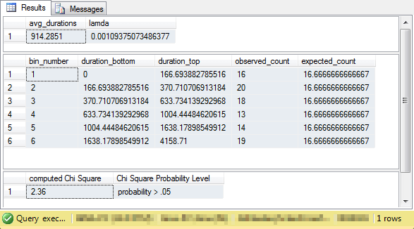
All the other code segments are unchanged from the preceding example in this tip. The following display shows the output from the full set of all five code segments. The two most important items are the computed Chi Square and the Chi Square probability level. Notice that the probability level is greater than .05. This means that the differences between the count of observed values per bin are not significantly different than the exponential distribution represented by the expected count values per bin. In other words, the SQL-based approach concludes it is safe to interpret source data as being derived from a population of values that are exponentially distributed.

The outcome from the Chi Square goodness-of-fit framework is consistent with the outcome reported by professor Winton. Neither the Chi Square goodness-of-fit framework nor the Kolmogorov-Smirnov test used by professor Winton rejects the null hypothesis that the interarrival times are exponentially distributed. However, the Kolmogorov-Smirnov test used by professor Winton transforms the raw data before testing instead of binning the raw data (as is the case for the Chi Square goodness-of-fit framework). This correspondence between the two tests along with the confirmation of the framework in the prior example verifies the robustness of the Chi Square goodness-of-fit framework. You can use it with substantial confidence for different kinds of data and with different counts and without the need to transform raw values and still get the same values as with other kinds of goodness-of-fit tests.

Before this section concludes, it may be worth numerically demonstrating the steps for the computed Chi Square within this example. These steps are displayed in the following excerpt from an Excel workbook for the observed counts (O_i) and the expected counts (E_i) in the preceding screen display. The results in rows 2 through 7 show the process for computing Chi Square components by bin. The computed Chi Square appears in cell F9 as the sum of Chi Square components across all bins in cells F2 through F7.

Comparing SQL Chi Square goodness-of-fit to maximum likelihood cell probability estimates

The maximum likelihood estimation for cell probabilities of unknown parameters is another technique for assessing goodness of fit. Professor Dan Sloughter of Furman college demonstrated this alternative approach in his lecture note titled Goodness of Fit Tests: Unknown Parameters. The technique Professor Sloughter demonstrated is sometimes referred to as the G-test (see here and here). This section briefly presents the data and main conclusions from Professor Sloughter's lecture note. Additionally, this tip contrasts the maximum likelihood estimation for cell probabilities of unknown parameters approach to the SQL-based Chi Square goodness of fit approach for the same data.

The following screen shot shows the lightbulb lifetimes as they appear in the lecture note. There are one hundred lifetime survival values in the source data. This data is similar in layout and structure to the microprocessor lifetime survival data used by professor Nygard in his lecture note. From a computational perspective, an important difference between the two approaches is how the lifetime values are grouped. The maximum likelihood estimation for cell probabilities of unknown parameters technique demonstrated by Professor Sloughter uses an ad hoc approach to grouping lifetime values for assessing if the lifetime data are drawn from a population of values with an exponential distribution. The SQL-based Chi Square goodness-of-fit approach bases the cell widths on the cumulative density function estimate for the data and the requirements for expected value minimums, average values, and number of categories (provided in Excel Master Series blog). Both approaches allow some flexibility in how to define categories or bins for grouping lifetime values.

The cell widths for the maximum likelihood estimation for cell probabilities of unknown parameters technique does not include any specific recommendations for cell widths that relate to expected counts by bin.
In contrast, the cell or bin widths for the SQL-based Chi Square goodness-of-fit framework must all have the same percentage based on the cumulative density function range, which is zero through one.
On the other hand, the ad hoc approach for the maximum likelihood technique does not have the requirement that the percentage of expected frequencies must be the same for all bins.

Professor Sloughter first groups lifetime values with an arbitrary cell width of 500. However, based on the low count of observed frequencies in some cells, he later re-groups several categories together into one bin so that the count of observed values in the freshly grouped set of bins is seven. This process reduced the total number of cells used with the maximum likelihood estimation for cell probabilities of unknown parameters technique from nine to six. After these modifications, the maximum likelihood approach confirmed that the exponential distribution provides a good description of the observed data.

The following display shows the original set of bin boundaries and counts from Professor Sloughter's lecture note. As you can see, the last four bins have especially small frequency counts.

Therefore, Professor Sloughter re-grouped the data into six bins. These bins along with the observed and expected counts appear next. Based on these re-grouped data, Professor Sloughter concludes that an exponential distribution provides a good fit to the observed data.

With the SQL-based Chi Square goodness-of-fit approach, the main requirements for the number of cells is that there are at least five cells and that the minimum expected value is at least one. Using the minimum of five bins results in an expected count of 20 per bin. By using a value of six bins to match the number chosen for use with the maximum likelihood estimation for cell probabilities of unknown parameters technique, the expected cell count reduces from 20 to 16.6666666666667. Therefore, the @total_bins variable that is set in the third SQL code segment must be set to six as in the second example and not eight as in the first example.

The original one hundred lifetime values were submitted to the SQL-based Chi Square goodness-of-fit framework. In one step, without any initial grouping and then subsequent manual re-grouping, the framework grouped the data and computed a Chi Square value that did not allow a rejection of the null hypothesis. As a result, the SQL-based framework also supported the assertion that an exponential distribution provides a good fit to the observed data.

The following excerpt from the output for the SQL-based framework shows the computed Chi Square value and its probability of occurring by chance. Because the probability of obtaining the computed Chi Square value is not statistically significant at the .05 level, it is concluded that the observed counts by bin are not significantly different than the expected counts by bin where the counts are based on an exponential distribution.

Instead of basing the bin boundaries on fixed increments for the observed counts range by bin, the SQL-based approach uses fixed increments of the cdf for the expected counts. Therefore, the boundary values for the SQL-based approach are not evenly spaced based on observed values. In contrast, the boundaries for the SQL-based approach are calculated so the expected count is the same for all bins because the expected probability from the cdf is the same for all bins.

Next Steps

This tip demonstrates in three sections how to assess if a set of values, including either lifetime survival durations or interarrival times, are drawn from a population of values with an exponential distribution. The SQL script files are slightly different as discussed in each section, and the data files with values are, of course, distinct from one section to the next. The script differences reflect variations in the layout of data values within a file and/or how many bins to use in assessing if data values are from a population of exponentially distributed values.

Additionally, an Excel workbook file contains a table of critical Chi Square values that the scripts use to automatically look up whether a computed Chi Square value supports a rejection of the null hypothesis. If the computed Chi Square value is not statistically significant with a probability level of least .05, then you can accept the null hypothesis that there is no difference between the input values and an exponential distribution of values. If you want to use the automatic statistical significance lookup feature in the SQL script files, then you need to import the workbook file into a SQL Server database and populate a corresponding SQL Server table as described in this tip. If you do not import the critical Chi Square values to a SQL Server table, then you'll need to comment out the code for the automatic statistical significance lookup feature.

The download file for this tip includes the seven files referenced in this section. After getting the three demonstrations to work as described in the tip, you should be equipped to participate in a data science project where you are charged with loading data values and assessing if they are drawn from a population of values that are exponentially distributed.

About the author

Rick Dobson is an author and an individual trader. He is also a SQL Server professional with decades of T-SQL experience that includes authoring books, running a national seminar practice, working for businesses on finance and healthcare development projects, and serving as a regular contributor to MSSQLTips.com. He has been growing his Python skills for more than the past half decade -- especially for data visualization and ETL tasks with JSON and CSV files. His most recent professional passions include financial time series data and analyses, AI models, and statistics. He believes the proper application of these skills can help traders and investors to make more profitable decisions.

This author pledges the content of this article is based on professional experience and not AI generated.

View all my tips