An Overview of Data Science for Stock Price Analysis with SQL: Part 1

By: Rick Dobson | Comments (1) | Related: > TSQL

Problem

Please provide an overview of data science focusing on time series data, such as for product sales or stock prices. I want the overview to be relatively broad and consider conceptual topics, but the overview should also tie back to prior tips with practical examples so that I can get a hands-on feel for doing data science via SQL programming.

Solution

This tip is the first in a two-part series that aims to empower SQL professionals to do data science. Special attention is given to time series data, namely stock prices. Although you can apply data science techniques to many different application domains, the domain to which you apply data science affects how data science is practiced. For example, facial recognition technologies are not important when projecting sales trends, but facial recognition technologies are widely used in some data science initiatives focusing on enhanced computer security.

The use of stock price and volume time series data for illustrating data science techniques is recommended for several reasons even if you never plan on trading stock securities.

Stock price and volume data are widely available for securities on a daily basis as well as historically over decades.
- There are thousands of securities for US companies, and more worldwide, that are traded daily on exchanges throughout the world.
- Many of these stocks have decades of historical data available for data science studies.
- Historical price and volume are available from many sources on a gratis basis or for a fee.
The data are easy to understand.
- Stock prices can go up and down.
- Volume complements price data. The more shares traded during a period, the more interest there is in a security among traders during that period.
- If a stock is bought when it starts rising and sold before it falls below the buy price, the stock trade earns a profit. A typical decision-making task is to identify a trade (a stock buy followed at some later time by a stock sale) which can earn a profit.
There is a rich body of technical analysis literature suggesting how to process historical stock price and volume data. This literature offers both a starting point for data science studies as well as a point of comparison for contrasting traditional stock technical analysis techniques with more recent and less domain-specific data science techniques.

This tip starts with an introduction to data science. Next, some commentary on technical analysis for time series data appears. This is followed by a discussion of some techniques for collecting historical stock price and volume data for input to an SQL Server database. Then, the tip shifts its focus to reviewing and highlighting how prior MSSQLTips.com tips illustrate data science techniques that you can implement with SQL.

The plan for the second tip in this series is to introduce and to review more data science topics and stock price indicators to help grow your data science capabilities for stock price analytics. This second tip is meant to highlight potential data science techniques that can be profitably addressed with SQL. The second tip in this series will definitely drill down on a prior tip that presented a starter kit for doing statistics with SQL. Extensions to the starter kit are likely to address determining the statistical significance of variables within a data set for more kinds of data and for different kinds of relationships than those initially presented, kinds of moving averages for time series data, and predictive analytics. There will also be some attention devoted to machine learning, such as an overview of machine learning, including decision tree analysis. Additionally, there will be coverage of additional stock technical indicators, including reading and interpreting candlestick chart data with SQL, volume-based indicators, and coverage of price support and resistance. Finally, the second tip in this series will also dive deeper into stock data collection for SQL Server databases and the testing of trading models for using the knowledge gained from data science for achieving trading gains.

What is data science?

There is substantial diversity of opinion on exactly what is data science. Rather than try to resolve divergent perspectives into the one true definition of data science, this tip refers you to other surveys of opinions about what is data science (Wikipedia and Quora). This tip also highlights selected features of data science as they relate to modeling when to buy and sell stocks for a gain.

The term data science is often used to refer to a convergence of programming, mathematics/statistics, and substantive knowledge in some domain area. Data science is different than its component elements in that it explicitly focuses on the interplay of programming, mathematics/statistics, and substantive knowledge instead of any one or two of these in isolation.

By programming, I mean using a computer to make sense of data in a way that often leads to decision-making about data. Python and R are two programming languages which are widely used in data science. SQL and NoSQL skills also apply equally well; both tool sets can help to save, process, and distribute the data in data science. Furthermore, proficient SQL and NoSQL developers can program classic data science techniques. Also, knowledge of how to manipulate a statistics or graphing package can also be thought of as programming in the context of data science. Even spreadsheet skills can be used profitably to facilitate some data science tasks.
By mathematics and statistics, I mean modeling and analyzing. You can use descriptive and inferential statistics to analyze data. Multiple linear regression analysis and logistic regression analysis are popular modeling tools, respectively, for continuous and discrete dependent variables. Yet another modeling tool is decision tree analysis. Clustering is a complementary statistically-based approach that is sometimes integrated with modeling. This integration involves grouping entities, such as persons or stocks, so that optimal models can be built for each group of homogeneous entities.
By substantive knowledge, I mean an application domain. Both weather forecasting and predictions for stock prices can involve time series data. However, the variables to use, the groups to track, and the conceptual structures for analyzing data over time are not the same across these two substantive areas.
- Specific knowledge about El Nino cycles, storm surges, and hurricane paths are important in weather forecasting but are not relevant to predicting stock prices.
- On the other hand, technical indicators, such as Relative Strength Indicator (RSI) and Moving Average Convergence Divergence (MACD) indicators, which are widely used to estimate stock price cycles have no relevance to weather forecasting.

What are stock technical indicators?

Stock technical indicators are tools for helping market professionals and traders to analyze historical stock price and volume data. This kind of data is available from many sources.

Yahoo Finance, and other websites, offers stock data available for free download.
You can also purchase it from various aggregator firms. For example, I received an email message recently from EODData (eoddata.com), with a claim it is "the # 1 site for End of Day Stock Market Data & History". If one site claims it is number one, then there must be many more in order to justify making the claim.
MSSQLTips.com offers a free SQL Server database (AllNasdaqTickerPricesfrom2014into2017) with nearly four years of price and volume history for NASDAQ exchange stocks. A link for downloading a backup copy of the database appears elsewhere within this tip.
The point is that stock market data are available from many different sources in lots of different formats.

Here is a screen shot with SQL code and sample historical stock price and volume data from the MSSQLTips.com database for NASDAQ exchange stocks. As you can see, the code extracts data for four symbols (MSFT for Microsoft Corporation, NFLX for Netflix Inc., GOOG for Alphabet Inc., and FB for Facebook Inc.) from the Results_with_extracted_casted_values table in the database. The data include standard historical price and volume data.

date - the trading date for other numeric values on a row
symbol - the symbol for representing a company's stock
open - the opening price for a stock
high - the high price for a stock
low - the low price for a stock
close - the closing price for a stock
volume - the number of shares traded

The data are displayed for the date range starting at 2017-10-30 through the row with the most recent date in the table for the stocks. The data were loaded while Yahoo Finance was in the process of updating the data for November 8, 2017. As a result, the data for that date can be missing and/or unreliable. For example, daily trading day data are provided for all four stocks, except on November 8, 2017 for the GOOG symbol, which did not have its data updated by Yahoo Finance for that date yet. Also, notice that the weekend days of November 4 and 5, 2017 are missing from the time series. Since these data are issued by stock markets, data is only available on days that the stock market is open for trading, which excludes weekend days and about ten holidays per year.

It is common for technical indicators to depend on one of two types of moving averages. These moving averages are sometimes used as technical indicators. A moving average represents an average value for a set of time series values, such as daily stock close prices.

The easiest moving average to compute is often referred to as a simple or arithmetic moving average. This type of moving is a running average of the last set of values in a time series. If you are computing a ten-period moving average, then it is the average of the last ten periods of time series data. One distinguishing feature of this kind of moving average is that you cannot have an arithmetic moving average value until enough periods are available to compute the first moving average. Therefore, you cannot compute a ten-period moving average until values for ten periods become available. See this prior tip for sample code and further discussion on how to compute with SQL arithmetic moving averages.
Another type of moving average is called an exponential moving average. The formula for the moving average is based on a recursive weighted function of the current period's time series value with the prior period's moving average. If the weight for the current period is represented by alpha, then the weight for the prior period's moving average is represented by 1 - alpha. There is no generally accepted standard among exponential moving average computers for a fixed number of prior period values to be available before the computation of the first exponential moving average. See this prior tip for sample code and further discussion on how to compute with SQL exponential moving averages.

The topic of moving averages for stock time series values is a very rich one. For example, there are other less commonly used types of moving averages besides arithmetic and exponential moving averages. Some analytic methods examine cross-overs in the values of two moving averages with different period values. Another approach that is sometimes used is examining if close prices remain above a moving average; dips of the close price below a reference moving average is commonly interpreted as a sign of price weakness. Other analytic methods take moving averages of moving averages to gain what are believed to be special insights. For reasons like these, it may be worth your time to become very familiar with moving average computational techniques if you plan on developing models for stock price time series values.

Given some historical price and volume data for a collection of stocks, you can compute and interpret technical indicators for the stocks. Any reasonably comprehensive list of technical indicators is going to be very long. Additionally, it is common for stock traders and analysts to adapt and extend indicators so that their implementation differs from when they were originally proposed. There are many websites and books from which to grow your knowledge of technical indicators. Here are a couple of links from Wikipedia and StockCharts that offer coverage of multiple classic and some not so classic technical indicators and related technical analysis tools for analyzing stock prices.

A primary goal of this tip is to present a handful of technical indicators that can be computed and/or used via SQL applications. All the selected technical indicators were covered in one or more prior tips. These prior tips focused heavily on how to compute technical indicators and assessing how they performed. Additionally, some of the prior tips identified weaknesses in an indicator as well as how to remedy weaknesses. Occasionally, the remedy involved modifying the computational process for one indicator so that it combined features from two or more different indicators.

Strategies for populating a table with stock close price values

In order to populate an SQL Server data table with historical price and volume time series data, you must

identify a source from which to obtain the data
import the data from that source into an SQL Server table

As mentioned in the preceding section, there are many sources from which to obtain historical price and volume data. One of the most comprehensive listing of these sources appears in this link. Many sources offer the data in exchange for a fee. One of the free sources is Yahoo Finance. Previous tips demonstrate different approaches to downloading historical data to an SQL Server table.

In my opinion, there is no single approach that works best for all situations, and it is my plan to re-visit the topic in the future to compare for a couple of scenarios different options for collecting historical price and volume data from Yahoo Finance and perhaps other sources. In the interim, I briefly highlight three prior articles here that demonstrate a couple of approaches for getting data from Yahoo Finance so that you can populate an SQL Server table with historical data.

My most recent attempts at gathering historical price and volume data from Yahoo Finance rely on using a Python-based programmatic interface to the Yahoo Finance site. Yahoo Finance and the maintainers of the Python language jointly agreed on how you can use Python to extract historical stock price and volume data from the Yahoo Finance site. One of my most straightforward tips on the basics of how the interface works appears in the following script; this tip is from a Simple Talk article.

The following screen shot shows an excerpt from the article. The highlighted section illustrates the use of the DataReader method from the panda_datareader library represented by an alias name of web. As you can see, the DataReader method takes four parameters.

The first parameter is for a stock symbol. The sample code designates the nvda symbol for Nvidia Corporation.
The second parameter designates yahoo to specify Yahoo Finance as the source from which to collect historical data.
The third and fourth parameters are variables whose values are assigned in prior assignment statements.
- The start parameter represents the beginning date for the collection of historical data.
- The end parameter represents the ending date for the collection of historical data.

The df variable represents a Python data container for a spreadsheet-like array of data; this array is referred to as a dataframe. The last statement in the Python script invokes the to_csv method for the dataframe object to save the collected data in the df object as a csv file in a default folder based on the folder from which the Python script file runs. Once the data are in a csv file, you can readily import them to an SQL Server table using your preferred method.

As attractive as the above script may be for its simplicity, it is not very practical for cases when you are working with historical price and volume data for many or even a modestly sized set of symbols. This other tip demonstrates a more robust approach for gathering historical stock price and volume data for thousands of symbols.

The approach illustrated saves in a text file thousands of symbols and related data items for stocks traded on the NASDAQ stock exchange; the data items originate from the NASDAQ stock exchange site. This step is accomplished with a Python script and a SQL script that interoperate.
Then, after some manipulation to account for the organization of the data, the data are imported into an SQL Server table.
Next, the symbols are extracted from the table and saved as a csv file.
Then, another Python script and another SQL Server script interact to directly copy historical price and volume data for the set of all NASDAQ stock exchange symbols available from the Yahoo Finance site. The data are staged to a temporary table as lines of text, which are the default output from Python print statements and functions.
Then, the lines of text are copied to another table. Additionally, the historical data in lines of text along with stock symbols are extracted to typed data columns in the Results_with_extracted_casted_values table within the AllNasdaqTickerPricesfrom2014into2017 database.

The following screen shot shows the design of the Results_with_extracted_casted_values table in Object Explorer.

The source data for the typed columns is in the line column, which has a type of varchar(500).
The open, high, low, close columns have a money data type, which is a standard one for representing stock price related data.
The date column has a date data type. The date column value represents the trading date for the other fields on a row.
The symbol column has a varchar(10) data type for holding a symbol. The maximum length is more than required for NASDAQ stock exchange symbols that never exceed five characters.

A sample query from this table and its result set appear in the preceding section. The following screen shot presents another query from the Results_with_extracted_casted_values table with both the source data column (line) and derived typed data columns (date, symbol, open, high, low, close, volume) for the first ten rows from the table ordered by symbol and date. This query and its result set illustrates the mapping of extracted fields from the source data to the typed data. More details on the transformation of text characters in the line column to other data types are described within the tip describing the initial population of the Results_with_extracted_casted_values table.

Golden cross and death cross indicators

The golden cross and death cross indicators are especially easy to understand technical indicators. You can compute them with either arithmetic moving averages or exponential moving averages.

The golden cross is a period (for example, a day) in which the fifty-period moving average moves from below to above the two-hundred period moving average. This transition is typically interpreted as buy signal for the stock. This is because the transition signals that recent stock prices as indicated by the fifty-period moving average are rising above less recent stock prices as indicated by the two-hundred period moving average.
The death cross is a period in which the fifty-period moving average moves from above to below the two-hundred period moving average. At this transition, recent stock prices are falling relative to less recent stock prices. If you have not already sold a position in a stock, the death cross can signal that you take that action.

This pair of technical indicators was examined in a prior tip that demonstrated how to detect golden crosses and death crosses based on either arithmetic or exponential moving averages with SQL. Twenty-seven stock symbols with at least one golden cross/death cross set of signals were selected for inclusion in this tip. These symbols were chosen for their convenient availability not because they were representative of a known population.

The tip relied on the mav_10_30_50_200 and ewma_10_30_50_200 tables in the AllNasdaqTickerPricesfrom2014into2017 database. The mav_10_30_50_200 table held arithmetic moving averages, and the ewma_10_30_50_200 table held exponential moving averages. You can create and populate these two tables in the AllNasdaqTickerPricesfrom2014into2017 database with scripts from prior tips ( this one for arithmetic moving averages; this other one for exponential moving averages). In fact, the prior tip for arithmetic moving averages provides a link for downloading a backup file for the AllNasdaqTickerPricesfrom2014into2017 database with the Results_with_extracted_casted_values table populated.

The main point of the tip on golden crosses and death crosses from a data science perspective is that buying at the golden cross and selling at the death cross can generate positive close change values. The tip aims to answer the question: is the sell close price on the recommended sell date greater than the buy close price on the recommended buy date. Some trades resulted in losses, but the median trade based on arithmetic moving averages resulted in a gain. This outcome reflects an interesting point about technical indicators. They can (often do) work some of the time but not all the time. Furthermore, the rules for trading with technical indicators need to be tested under different scenarios because there may be special setup conditions that determine how best to use a technical indicator.

The following table excerpted from the tip on golden and death crosses presents some summary findings for the performance on multiple metrics of death crosses with arithmetic moving averages versus exponential moving averages.

The golden cross/death cross pairs generated their best trading results when based on arithmetic moving averages as opposed to exponential moving averages. For example, the percent of up trading days in buy/sell cycles was 92 percent when they were based on arithmetic moving averages, but only 65 percent when based on exponential moving averages.
Also, trades based on the arithmetic moving average had a median percent gain of 12 percent in close price versus a 5 percent loss for trades based on an exponential moving average.
As a result, you should use arithmetic instead of exponential moving averages when recommending buy/sell dates using golden cross and death cross pairs.
Even for the type of moving average that worked best, the golden cross/death cross pairs did not return 100 percent winning trades. One reason for this is because the decline in the fifty-period moving average at the end of buy/sell cycle can exceed earlier gains in the buy/sell cycle.
If you were to settle on using golden cross/death cross cycles for buy and sell signals, additional research may be merited on how to select an earlier sell signal than the death cross. This recommendation follows from casual observation that the percent gain can drop drastically as the fifty-period moving average declines in the direction of the two-hundred period moving average.
More thoughtful sample selection may also be warranted so that the results can be readily extrapolated to some known population of stocks. The sample of stocks for the tip introducing golden crosses and death crosses used a selection of symbols that was quick and easy to compile.

Moving average convergence divergence Indicators

The moving average convergence divergence (MACD) indicators are a set of three coordinated stock technical indicators.

The core MACD indicator is typically referred to as the MACD line indicator. The MACD line value reflects the convergence or divergence between two exponential moving averages.
- The first moving average is a shorter-period one; a period length of twelve days is commonly used.
- The second moving average is a longer-period one, a period length of twenty-six days is commonly used.
- As the difference of the shorter-period moving average less the longer-period moving average approaches zero, the two moving averages converge. This can happen either because the shorter-period moving average rises from below to above the longer-period moving average or because the shorter-period moving average falls from above to below the longer period moving average.
- As the shorter-period moving averages nears the longer-period moving average, the two moving averages converge.
- As the difference of the shorter-period moving average less the longer-period moving average grows, the values of the two moving averages diverge from one another.
The signal line indicator is an exponential moving average of the MACD line values. When twenty-six-period and twelve-period moving averages are used to compute the MACD line values, then a nine-period moving average of the MACD line values is typically used to compute the signal line.
The third MACD indicator is referred to the MACD histogram value.
- The signal line values are often plotted on the same chart as the MACD line values.
- The MACD histogram indicator is the MACD line value less the signal line value.
- The MACD histogram indicator receives the name MACD histogram because its values are often plotted as histogram bars above and below the centerline or zero-line value for the MACD line chart.
There are two types of MACD technical indicator crossovers that are used as signals for when to buy and sell stocks. The MACD line can cross above or below either its centerline value of zero or it can cross above or below its signal line value.
- Centerline crossovers can be either of two types. These crossovers indicate a change in direction of underlying stock prices.
  - When the MACD line crosses the centerline value of zero to become positive, this indicates that more recent stock prices are rising faster than less recent stock prices. This upward momentum in stock prices indicates a good time to buy a stock.
  - When the MACD line crosses the centerline value to become negative, this indicates that more recent stock prices are falling relative to less recent stock prices.
- Similarly, signal line crossovers can be either of two types. These crossovers signal a likely future change in the direction of underlying stock prices.
  - When the MACD line value crosses above the signal line value even if it is below zero, then it is also sometimes viewed as a buy signal. This is because shorter-period moving averages are trending up even if they are not yet above longer-period moving averages.
  - When the MACD line value crosses below the signal line value even if it is above the zero MACD line value, then it is also sometimes viewed as a sell signal. This is because shorter-period moving averages are trending down. If they continue on this trajectory, shorter-period moving averages will fall below longer-period moving averages.

Here are two prior tips that drill down specifically on MACD indicators for data scientists using SQL as well as a good general introduction to the indicators.

The first tip focuses on demonstrating how to compute the three MACD indicators.
- In fact, its main value is to populate a table with the three MACD indicators for every eligible trading date in the macd_indicators table of the AllNasdaqTickerPricesfrom2014into2017 database.
- The first tip on the MACD indicators also performs some analysis on a sample of symbols chosen for convenience purposes to verify if a stock's close price increases from the date that the MACD line value crosses from below to above its centerline value to the date that the MACD line value falls from above to below its centerline value.
The next MACD tip switched the focus from introducing the MACD indicators to a couple of data science techniques.
- First, there were two samples of symbols in the second tip. These symbols were selected according to rigid criteria so that while the symbols were different in each sample, they were chosen from a common pool of similar symbols. This similarity made it possible to reliably test for the consistency of results over both samples.
- Second, models were built for estimating the close change from yesterday on either
  - MACD histogram change from yesterday or
  - MACD line value change from yesterday
- These models were estimated fore each sample, and then run in the other sample. Goodness of fit measures verified the ability of the sample for one model to predict close change values for the other sample. This is a standard data science technique commonly called cross-validation.
If you seek a good general introduction to the MACD indicators that is not specifically tied to SQL calculations or model development, then I recommend this StockCharts tip.

The following screen shot shows an Object Explorer view of the macd_indicators table. By placing the close price value in the macd_indicators table, you facilitate unit testing the computed values in the macd_indicators table based on the source data from the Results_with_extracted_casted_values table. It is also convenient to have the close price in the macd_indicators table for accounting purposes in relating MACD indicator values to close prices.

Over the nearly four years of history in the AllNasdaqTickerPricesfrom2014into2017 database, the number of MACD centerline crossover start and end dates varies somewhat from symbol to symbol. The following screen shots shows start date and end date for the thirteen pair MACD centerline crossovers for the MSFT symbol.

In addition to the dates, symbol, MACD line value (macd), several other fields are displayed.
These additional fields include
- Number of trading days (number_of_row_number)
- Close price on the first day of an MACD cycle (close_first)
- Close price on the last day of an MACD cycle (close_last)
- The maximum close price within a cycle (clase_max)

As you can see, the close_last column values are generally greater than the close_first column values. This confirms the ability of the MACD line value and centerline crossovers to identify sell prices that are typically higher than their buy price. For seven of thirteen MACD centerline crossover cycles for the MSFT symbol, the sell close price exceeds the buy close price. The same pattern held up for most of the other symbols examined in the first tip for MACD indicators. Over the set of 10 symbols used in the first MACD tip, the sell close price was larger than the buy close price to confirm the tendency of close prices to rise during MACD cycles.

The second tip targeting MACD indicators looked at a matched pair set of symbols. Symbols were selected so that they represented investment grade companies with a lot of data in the AllNasdaqTickerPricesfrom2014into2017 database. Then, symbols were ordered by the size of the change in close price from their first trading date in 2014 through their last trading date in 2017. Finally, the top twenty symbols were split into two matched halves of ten symbols each. Odd symbols had order numbers of one, three, five, etc., and even symbols had order numbers of two, four, six, etc.

Next, MACD cycles were computed for each symbol within each set of symbols. Within each symbol in a set, MACD cycle start dates were computed, and data were collected for the next twenty trading dates as well. Each of the twenty trading dates after the start date was classified by two variables.

For the macd_gt_0 column value,
- a trading date was assigned a value of one if the MACD line value was greater than zero
- else a trading date was assigned a value of zero if the MACD line value was not greater than zero
For the macd_gt_signal column value,
- a trading date was assigned a value of one if the MACD line value was greater than the signal line value
- else a trading date was assigned a value of zero if the MACD line value was not greater than the signal line value

The two-way classification of the macd_gt_0 and macd_gt_signal column values were assigned names to denote whether it was a good time to own a stock. Then, SQL code was run to compute the change in close value from the first trading date in MACD cycles through each of the remaining twenty days. An outer query computed the average close change value and count of each combination of macd_gt_0 and macd_gt_signal values. The results were then copied to an Excel workbook for the calculation of additional summary results.

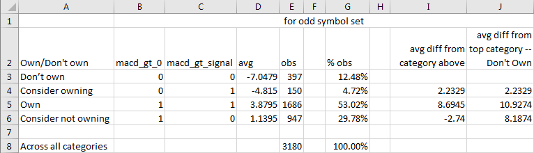
The following table shows the results for the odd symbols. The same set of computations are available in the tip for even symbols.

Column A specifies a name for whether it is a good time to own a stock based on the two-way classification of macd_gt_0 and macd_gt_signal values for a trading date; these values appear in columns B and C.
When the macd_gt_0 column value and macd_gt_signal column value for a trading date both equal 1, it is a good time to own a stock. On these trading dates, the average close change value rounded to the nearest penny is $3.88 more than on the first trading date in an MACD cycle.
When the macd_gt_0 column value and macd_gt_signal column value for a trading date both equal 0, then it is a good time to not own a stock. On these trading dates, the average close change value rounded to the nearest penny is $7.05 less than on the first trading date in an MACD cycle.
The change in average close price rounded to the nearest penny is $10.93 between the Own category trading days and the Don't own category trading days.
Clearly, whether the MACD line value is greater than zero and whether the MACD line value is greater than the signal line value have a big impact on the close change value from the first day in a MACD cycle.

Several linear regressions were run for predicting change in close price from yesterday based on either of two other variables. The model that worked best was a model for predicting change in close price from yesterday based on change in MACD histogram value from yesterday; recall that the MACD histogram value is the MACD line value less the signal line value. The model had about the same slope and intercept value for the odd and even set of symbols. Furthermore, the coefficient of determination for the regression model was about the same (.86) in both samples of symbols.

The most striking outcome came from the running of cross-validation tests. A cross-validation test involves running the model trained on one set of values on another sample of values. In the cross-validation tests for the tip, the linear regression model developed for the odd sample was run with the data for even sample and vice versa. Both cross-validation tests yielded results that confirmed that each model trained in one sample worked about equally well in the other sample!

The relative strength indicator

The RSI (relative strength indicator) compares price gains to price losses over a recent window of trading periods. In this tip, we are focusing on periods with a duration of one trading day, but there is nothing in the RSI that restricts it for use with a period equal to one trading day. It is common to use a window length of fourteen periods, but traders and analysts sometimes use different windows with more or less periods per window. In this tip, we are using the common window length of fourteen.

Three prior tips address the RSI in ways that are relevant to this tip.

An initial tip introduces the RSI to SQL developers, demonstrates how to populate a table of RSI values for trading dates in the AllNasdaqTickerPricesfrom2014into2017 database, and does some preliminary analysis on how the RSI performs.
Another tip demonstrates how to address an issue with the RSI for designating the end of buy/sell cycles and compares results before and after the fix.
A third tip does a comparative analysis of the RSI with and without the fix for designating the end of buy/sell cycles as well to other models for designating buy/sell cycles.
For those who care to dig more deeply into the RSI from a non-SQL programming perspective, you can examine these articles from StockCharts and Wikipedia.

The RSI targets price reversals. That is, it aims to tell when a trend of increasing prices starts falling from overbought price levels. Likewise, the RSI also can indicate when prices initially move above oversold levels. For these reasons, RSI values can range from 0 (for completely oversold) through 100 (for completely overbought). If your goal is to tell when to buy and sell a stock based on RSI values, it is common to use two cutoff values.

For a buy signal, traders and analysts use a migration from an RSI below thirty to a value above thirty.
For sell signal, traders and analysts often use a migration from an RSI above seventy to a value below seventy.

The following screen shot from the first SQL-based RSI tip shows a succession of migrations between overbought and oversold RSI value levels for the NVDA stock symbol in the AllNasdaqTickerPricesfrom2014into2017 database. The NVDA symbol represents the Nvidia Corporation.

Rows with a yellow background denote the first date within a buy/sell cycle when the RSI value moves from an oversold to a non-oversold level. This type of RSI value transition marks the beginning of a buy/sell cycle. As you can see, there are three starts for NVDA buy/sell cycles.
- The first is on October 14, 2014 when the RSI value migrates from 23.477 to 32.268.
- The second is on July 10, 2015 when the RSI value changes to 36.671 from 29.194.
- The third is on January 21, 2016 when the RSI value moves to 31.568 from 28.505.
Rows with the term "leaves oversold" in the F column without any background color denote an instance when the RSI indicates a reversal from a non-oversold level to an oversold level and back again to non-oversold level. There is only one instance of this kind of reversal for the NVDA symbol. This kind of "leaves oversold" reversal concludes on February 12, 2016.
Rows with a green background denote the first date within a buy/sell cycle when the RSI value moves from an overbought to a non-overbought level. This type of RSI value transition marks the traditional end of an RSI buy/sell cycle. Again, there are just three traditional ends in the sample data below.
- The first is on November 7, 2014 when the RSI value changes to 63.21 from 71.502.
- The second is on August 18, 2015 when the RSI migrates to 67.6 from 72.727.
- The third is on March 3, 2016 when the RSI moves to 67.45 from 70.054.
Rows with a rose background identify the last date after a preceding buy/sell start in which the RSI moves from an overbought level to a non-overbought level. These rose background rows mark dates after the traditional end of an RSI buy/sell cycle when the RSI makes its last move from overbought to non-overbought values. There are three rows with a rose background - one corresponding to each of the traditional buy/sell cycles.
- The first is on February 18, 2015 when the RSI value moves to 67.128 from 71.287.
- The second is on December 9, 2015 when the RSI changes to 62.17 from 70.59.
- The third is on September 21, 2017 when the RSI migrates to 61.699 from 70.165.
Rows with the term "leaves overbought" in the F column without any background color denote a reversal from a non-overbought level to an overbought level and back to a non-overbought level. This kind of reversal occurs after the first "leaves overbought" record with a green background marks the end of a traditional buy/sell cycle and before the last "leaves overbought" record following a preceding buy signal. There is at least one "leaves overbought" record corresponding to each NVDA buy/sell cycle.
- The first buy/sell cycle has just one "leaves overbought" row in the F column without any background color.
- The second buy/sell cycle has four "leaves overbought" rows in the F column without any background color.
- The third buy/sell cycle has twenty "leaves overbought" rows in the F column without any background color.

When a "leaves overbought" record initially occurs after the start of a buy/sell cycle, the RSI marks the end of a time of rising stock prices. Therefore, it is a good time to sell a stock then because prices were generally rising before this trading date. On the other hand, as the number of subsequent "leaves overbought" records grows before the first "leaves oversold" record for the start of the next cycle, then selling at the first "leaves overbought" record can cause substantial stock price gains to be missed.

Because of the possibility of missed gains by selling at the first "leaves overbought" record, it is worthwhile seeking an alternative sell date which will capture more gains from subsequent "leaves overbought" records after the first "leaves overbought" record in a traditional RSI buy/sell cycle. For example, the following screen shot shows that the first "leaves overbought" gain across all three buy/sell cycles is 19.86 percent for selling at first "leaves overbought" record. However, this percent gain can grow to 263.96 percent if sold on the last "leaves overbought" record before the start of the next buy/sell cycle!

The macd_gt_0 and macd_gt_signal fields from the preceding section can help indicate when it is no longer a good time to continue holding a stock. Instead of using the traditional first "leaves overbought" RSI record to end a buy/sell cycle, you can end a cycle based on the macd_gt_0 and macd_gt_signal field values confirming it is no longer a good time to hold a stock. Casual inspection suggested using the second of two consecutive periods with macd_gt_0 and macd_gt_signal field values both equal to zero.

A follow-up tip to the first SQL-based RSI tip performs a comparative analysis of RSI buy/sell cycles ending with the traditional first "leaves overbought" record versus the confirmed macd-based indicators that it is no longer worth holding a stock. This follow-up tip performed the comparison for an initial six-stock set of symbols used in the first SQL-based RSI tip and an additional two hundred forty-two investment grade set of stocks. For both sets of stocks, the macd-based indicators generated statistically significant greater gains during buy/sell cycles than the traditional first "leaves overbought" signal for ending a cycle.

Comparing and combining artificial intelligence models

The models discussed in this tip so far illustrate simple examples of what some may call artificial intelligence. The use of technical indicators provides a basis for calculations that result in recommendations about when to buy and sell stocks. The model-based buy and sell dates are a kind of artificial intelligence that can complement or replace human decision-makers making recommendations about when to buy and sell stocks.

From a data science perspective, the modeling/analysis described at the end of the preceding section for replacing the RSI-based sell dates with MACD-based sell dates is especially interesting. This is because all three aspects of data science interplay with one another.

Initially data mining uncovers a weakness of the traditional RSI indicator for defining sell dates.
Then, modeling analysis and SQL code are used to derive a new modified model that replaces the traditional RSI-based sell dates with MACD-based sell dates.
Finally, statistical tests are used to assess whether the MACD-based sell dates generate superior gains to RSI-based sell dates.

This section drills down on another tip featuring data science through comparisons of five models based on three different types of technical indicators. In fact, the models are compared with one another via a data mining activity. Additionally, the mined results are used as a basis for combining two of the initial five models into a new, combined model. Instead of combining at the level of technical indicator components, this section illustrates combining at the level of non-overlapping buy/sell cycles.

The following table presents the top line comparison results for the five initial models. You are familiar with the first four models because this tip explicitly covered them in previous sections. The fifth model was not explicitly discussed, but you will discover that you are familiar with its core features.

The model names appear in the source column.

macd cycles ending below centerline is the name for a model with
- a buy signal when the MACD line value crosses from below to above the centerline value of zero
- a sell signal just before the MACD line value crosses from above to below the centerline value
macd cycles ending below signal line is the name for a model with
- a buy signal when the MACD line value crosses from below to above the centerline value of zero
- a sell signal just after the MACD line value crosses below the signal line value
rsi cycles with macd ends is the name for a model with
- a buy signal when the RSI value rises from below to above 30
- a sell signal based on the second consecutive trading date with macd_gt_0 equal to zero and macd_gt_signal equal to zero; value assignments for the macd_gt_0 and macd_gt_signal column values appear in the "Moving average convergence divergence Indicators" section
rsi cycles with rsi ends is the name for a model with
- a buy signal when the RSI value rises from below to above 30
- a sell signal when the RSI value falls from above to below 70
trend up trades is the name for a new model based on four exponential moving averages having period lengths of ten, thirty, fifty, and two hundred with
- a buy signal when each shorter-period moving average close price is initially greater than its longer-period moving average close price for a contiguous block of trading dates
- a sell signal when any of the shorter-period moving average close price values is less than a longer-period moving average close in a contiguous block of three or more periods
- this model is initially discussed in a tip titled "Using SQL to Quantify Trend Direction and Strength"
- then, the model is further refined for buy and sell signals in a subsequent tip

Here's a summary of key findings from the preceding table.

The sum of the close price change amounts for a model is simply the sum of the sell price less the buy price for each buy/sell cycle associated with a model.
- All five models based on technical indicators generated a close price gain across all buy/sell cycles for a model.
- The trend up trades model generated the largest overall gain; the requirement for successively larger moving average values as the period length shrinks is the best model for detecting overall gains.
- The macd cycles ending below signal line model had the lowest gain, but the macd cycles ending below centerline model had the second highest gain. Selling when the MACD line value falls below signal line crossover apparently misses some gains that occur after the signal line but before the MACD line value falls below zero.
- It may be worth noting that the macd cycles ending below signal line model generates better gains for intermediate length cycles, which do not offer enough trading dates for the MACD cycles to generate their best gains.
Not all models generated the same number of buy/sell cycles; the count of cycles column values shows the number of buy/sell cycles associated with each model. By dividing the sum of close change amount column value from the preceding table by the count of cycles, you can calculate a quantity representing the average change amount per buy/sell cycle.
- The two rsi models generated the fewest number of buy/sell cycles.
- Although the trend up trades model generated the largest positive overall close change amount value, it did not generate the greatest positive overall close change amount value amount per buy/sell cycle.
  - The average gain per buy/sell cycle for the rsi cycles with macd ends model is $30.58 per share.
  - On the other hand, the average gain per buy/sell cycle for the trend up trades model is just $10.11 per share.
- Nevertheless, the overall gain for the trend up trades model is more than thirty percent greater overall than for the rsi cycles with macd ends model. This is because there are many more trend up trades buy/sell cycles than rsi cycles with macd ends buy/sell cycles.
Another comparison metric of particular interest is the value in the column named "prct source gt_20 column". This name denotes the percent of buy/sell cycles with a close change percent value that is greater than twenty percent more than the buy close price.
- These larger change percent values were sometimes much larger than other change percent values for gains.
- As a result, a relatively small percentage point advantage for the larger gains could significantly impact the overall gain for a model.
- This kind of outcome appears to account for the larger overall gain amount for buy/sell cycles from the rsi cycles with macd ends than for the rsi cycles with rsi ends.

Based on the preceding results, the outcomes from the trend up trades model were combined with the rsi cycles with macd ends model. The process of combining the two models required special attention because some trading dates could be associated with business cycles for both models. If any of the trading dates from a trend up trades business cycle overlapped with the trading dates from a rsi cycles with macd ends business cycle, then the trading dates from the cycle were assigned to the rsi cycles with macd ends model. Recall that the rsi cycles with macd ends model had a much greater gain per business cycle than the trend up trades model. The details of how to combine the two models with SQL are described here.

The following table compares the new combined rsi cycles with macd ends/trend up trades model to its two constituent models in the next screen shot depicting a comparison table between all three models.

The new combined rsi cycles with macd ends/trend up trades model has the name rsi macd end and non_overlap trend up in the source column.
The most important outcome is that sum of close change amounts for the new combined model is just over twenty-eight percent greater than for the trend up trades model. This outcome is especially significant because the trend up trades model has the greatest close change amounts total of any of the initial five models.
Also, slightly more than fifty percent of the new combined model buy/sell business cycles result in gains.
Based on these outcomes additional research is warranted to verify if the superior outcome for the new combined model with a sample of ten symbols extrapolate to different samples of symbols.

Next Steps

There are no original scripts associated with this tip. Instead, this survey tip relies on prior MSSQLTips.com tips exploring how to model recommended buy and sell dates for stocks. Additionally, several other links are provided to help readers increase their knowledge of data science, stock technical indicators, and the collection of historical stock price and volume data.

Here is a list of the links for prior tips from MSSQLTips.com in this survey tip.

Here is a list of the links from other sites referenced in this survey tip.

I close by indicating that this tip is not offering financial advice for any particular stocks or any specific trading rules; any recommendations are offered as data science observations about the outcomes surveyed in this tip. The stocks appearing in this tip were selected based on multiple objective business rules and/or personal choice depending on the tip being surveyed. At the time that I submitted this tip to MSSQLTips.com, I and my family members held positions in a subset of these stocks. I do occasionally use selected technical indicators, including the MACD, RSI, and multiple moving average indicators in making decisions about which stocks to trade, but I do not routinely use the precise trading rules covered in this tip.

About the author

Rick Dobson is an author and an individual trader. He is also a SQL Server professional with decades of T-SQL experience that includes authoring books, running a national seminar practice, working for businesses on finance and healthcare development projects, and serving as a regular contributor to MSSQLTips.com. He has been growing his Python skills for more than the past half decade -- especially for data visualization and ETL tasks with JSON and CSV files. His most recent professional passions include financial time series data and analyses, AI models, and statistics. He believes the proper application of these skills can help traders and investors to make more profitable decisions.

This author pledges the content of this article is based on professional experience and not AI generated.

View all my tips

Tuesday, May 7, 2019 - 5:07:38 AM - data science trainging in hyderabad	Back To Top (79968)
good article about data science thank you.