K Nearest Neighbor TSQL SQL Server Example

By: Rick Dobson | Comments | Related: > TSQL

Problem

I am looking for T-SQL code to implement the K nearest neighbors (KNN) algorithm. I want to get a first-hand feel for the algorithm's logic for classifying objects because I recently joined a data science team and wanted to see if this could be implemented in SQL Server with T-SQL.

Solution

This is the first part in a four-part series on coding data science algorithms with T-SQL. As indicated by the Problem statement, this part focuses on how to classify objects via the KNN algorithm. All four parts, and especially this first part, focus on the basics of implementing data science algorithms.

The KNN algorithm applies a "birds of a feather flock together" rule for assigning classifications to the objects in a set. The rule's name implies that birds of the same species fly close together in a flock. Another example of the objects in a KNN application can be persons who are candidates for having only heart disease, only diabetes, heart disease and diabetes, or neither heart disease nor diabetes. Test results can yield objective scores of various symptoms for each person in a data science project. If you know the objective scores and symptoms and the classifications of persons, you can use the KNN algorithm to assess if the objective scores and symptoms correctly classify persons.

The KNN algorithm can be used to assign classifications to a wide range of object types. For example, this tip uses a set of time series instead of a set of persons or birds. Each time series object has price values for two different types of securities. The time series objects are known to belong to two different groups. For one group of time series, the price of one security type moves up while the other security type moves down. In the second time series group, the security type price that rises in the first group falls in the second group, and the security type price that falls in the first group rises in the second group. This tip's KNN application assesses whether a collection of eight time series with two security types each can be reliably differentiated based on security price movements.

An introduction to the KNN algorithm

The KNN algorithm starts by specifying the objects in a set. As indicated in the Solution statement, the objects may be persons or time series or bird species that may flock together based on a distance metric. Indeed, the objects can be any set of entities that are distinct, such as customers, stores, or countries.

When using the KNN algorithm for classification, then each object should have both a known classification as well as test results that may be related to the classification types. For example, each person in a data science project for diagnosing illnesses may belong to one of four clusters: only heart disease, only diabetes, heart disease and diabetes, or neither heart disease nor diabetes. Each person also needs test results and observations that may indicate to which classification a person belongs.

Next, the KNN algorithm computes the pairwise distances based on test results and observations between the objects in a set. The distances between the members of each pair depends on the test scores and observation for each object. There are several different approaches for computing the distances between the members of each pair. This tip uses the Euclidean distance formula for computing the difference between objects. This link explains and contrasts several different kinds of distance metrics.

Next, you should examine the K nearest neighbors that belong to the same classification.

When K equals 1, then the KNN algorithm classifies each individual object as belonging to the same classification as the object that is closest to it.
When K equals more than 1, then the KNN algorithm classifies each object as belonging to the most common group among the K closest objects. In other words, the majority classification among the K nearest objects is assigned to the comparison object. Because of this majority wins rule, you should use values of K with classifications that have an odd number of possible outcomes.

Finally, you can compare the estimated classifications for a set of objects for different values of K to the known classifications for a set of objects. Ignoring the problem of overfitting, the matches across all objects between estimated classifications and known classifications should be perfect or as high as possible.

The data for this tip

This tip tracks price changes for two types of ETF securities over a set of eight different time series. ETF securities resemble mutual funds in some ways, but they can be bought and sold as conveniently as individual company stocks.

The ETF securities whose prices are tracked in the time series of this tip seek investment results which are based on the S&P 500 index or the NASDAQ 100 index. The S&P 500 index tracks all 500 stocks in the S&P 500. The NASDAQ 100 index tracks just the securities issued by 100 of the largest non-financial companies listed on the NASDAQ stock exchange.

A regular ETF moves up and down in price as the index on which it is based moves up and down. An inverse ETF moves up and down in price inversely to the index on which it is based. As you can see, inverse and regular ETF securities can trend in opposite directions over a time series. This tip specifically tracks four ETF securities.

The SPY is a regular ETF that tracks the S&P 500 index. Changes in the SPY price are positively correlated with the changes in the S&P 500 index.
The SH is an inverse ETF that also tracks the S&P 500 index. Changes in the SH price are inversely correlated with the changes in the S&P 500 index.
The QQQ is a regular ETF that tracks the NASDAQ 100 index. Changes in the QQQ price are positively correlated with the changes in the NASDAQ 100 index.
The SQQQ is an inverse ETF that also tracks NASDAQ 100 index. Changes in the SQQQ price are inversely correlated with the changes in the NASDAQ 100 index.
- The SQQQ is also a leveraged ETF so that changes in the SQQQ price are -3 times those in the NASDAQ 100 index.
- The other three ETF securities that this tip tracks are non-leveraged ETF securities meaning that changes in the security's price are 1 times their corresponding index change for regular ETF securities (SPY and QQQ) or -1 times the S&P 500 index for the other inverse ETF security (SH).

This tip relies on eight distinct time series. These series are named based on three criteria:

the securities tracked in the time series
the year containing the trading dates
whether regular ETF prices rise relative to inverse ETF prices (reg ETF wins) or whether regular ETF prices decline relative to inverse ETF prices (inv ETF wins)

The names for the time series in this tip are as follows:

SQQQ and QQQ 2011 inv ETF wins
SH and SPY 2011 inv ETF wins
SH and SPY 2019 inv ETF wins
SH and SPY 2020 inv ETF wins
SH and SPY 2010 reg ETF wins
SQQQ and QQQ 2020 reg ETF wins
SH and SPY 2020 reg ETF wins
SH and SPY 2019 reg ETF wins

The following screen shot is from an Excel worksheet that displays the data and some supporting data mining results for the SH and SPY 2020 reg ETF wins time series.

This worksheet is a component in the "Price changes for regular and inverse etfs.xlsx" workbook file. The workbook is available in the download for this tip.
The closing prices for the SH ETF appear in rows 2 through 9 of column C.
- The relative price change from 4/1/2020 appears in rows 3 through 9 of column B. As you can see, the ETF price drops over the time series from .97 for 4/2/2020 through to .88 for 4/13/2020.
- Sh prices are generally declining throughout the time series. The chart to the right of rows 2 through 9 shows the path of the declining relative prices.
The closing prices for the spy ETF appear in rows 16 through 23 of column C.
- The relative price change from 4/1/2020 appears in rows 17 through 23 of column B. For this regular etf, the relative prices generally increase over the time series.
- The path of the increasing relative prices appears in the chart to the right of rows 17 through 23.
Once the relative price changes for spy and SH ETF securities are computed, they are copied, respectively, to rows 33 through 39 of columns B and C. The relative price changes of sh_change_percent_from_start versus spy_change_percent_from_start appears in the chart to the right of the two sets of relative changes. This chart confirms that the spy relative prices increase from the beginning to the end of the time series while the SH relative price changes decrease from the beginning to the end of the time series.
Next, the differences between the relative prices for spy and SH ETF securities are computed and displayed in rows 44 through 50 of column C.
The bottom chart in the worksheet displays the SH relative price changes versus the spy relative price changes in a regression plot.
- As you can see, the plot has a negative slope, which illustrates the inverse relationship between SH relative prices and spy relative prices.
- The coefficient of determination (R²) is almost 1. This indicates that the line explains nearly all the variance between the two sets of relative prices.
The average of the relative price differences is computed in cell C52 with Excel's average function. The cell address and the expression illustrating the use of the average function appears directly above the body of the worksheet.

The same data mining steps are applied to each of the remaining time series for this tip. The following screen shot displays the summary results section of the worksheet for the SH and spy 2020 inv ETF wins time series.

The spy and SH relative differences appear in rows 66 through 90 of columns B and C, respectively. The base closing value for computing relative values is 2/14/2020. As a reminder, this date appears in row 65 of column A.
The top chart to the right shows the SH relative prices growing over the extent of the time series while the spy relative price changes decline.
This pattern is the reverse of the one in the preceding worksheet. The rising SH relative prices confirms the inv ETF wins classification for this time series.
The differences between the relative differences show in rows 95 through 119 of column C.
The second chart to the right shows SH relative price values versus spy relative price changes.
- The regression of SH relative prices on spy relative prices again results in a nearly straight line with an R² value of nearly 1.
- AAlso, the slope is close to -1, which confirms an inverse relationship between relative prices of the SH ETF versus the spy ETF in a different time series than the one shown in the preceding worksheet.

Classifying and Verifying Object Assignments to Groups

Recall that the objective of the KNN algorithm is to assign objects to groups based on different values of K. The computed group assignment is based on the proximity of an object to each of the other objects in a set. The computed group assignment is the group of the closest object to the object for which you are computing a group assignment. Therefore, you need to know two things to develop computed group assignments: the group for each object in a set and the distance between all pairs of objects in a set. The K in the KNN algorithm designates the number of objects for which you compare pairwise distances. Recall from the "An introduction to the KNN algorithm" section that:

the computed group assignment is based on the comparison of each object to each other individual object when K equals 1
when K equals more than 1, then each group is compared to two or more other objects
- the group assignment for values of K greater than 1 depends on a majority wins rule.
- therefore, if you have two groups to which to assign objects, you can perform three comparisons and assign the group that matches the test object two or more times

After you derive computed group assignments, then you can compare the computed group assignment to the actual group to which each object belongs. The minimum value of K that has the greatest correspondence between the actual group to which objects belong and the computed group assignment for objects is the best K for assigning objects to groups.

Insert the objects in a table for computing inter-object distances

The following script inputs the data for the eight time series objects in this tip.

The script starts by declaring DataScience as the default database, but you can use any other database of your choice.
The time series id, time series name, group name, and average of differences are specified as column names in the reg_and_inverse_etfs_for_knn table.
- The time_series_id and time_series_name values identify each of the time series in this tip with either a number or a name.
- The group_name values specify one of two groups.
  - TThe group named inv ETF wins is for time series with rising inverse ETF prices and declining regular ETF prices.
  - The group named reg ETF wins is for time series with a rising regular ETF prices and declining inverse ETF prices.
A set of select statements and union operators specifies values for the time series in this tip. An insert into statement populates the reg_and_inverse_etfs_for_knn table with the concatenated set of rows from the union operators.
The select statement at the end of the script displays the values in the reg_and_inverse_etfs_for_knn table. The average_of_differences from this table provides a single number that characterizes the relative direction of inverse and regular ETF prices in each of the time series. The average_of_differences provides a metric for computing the distance between the time series. This metric can, in turn, be used to compute the pairwise difference between objects.

use DataSciencego
 
-- create table to hold classification data
 
-- Remove prior reg_and_inverse_etfs_for_knn
if exists (select * from  sys.objects 
         where name = 'reg_and_inverse_etfs_for_knn' and TYPE =  'u')
    DROP TABLE dbo.reg_and_inverse_etfs_for_knn
 
 
create table dbo.reg_and_inverse_etfs_for_knn
(
Time_series_id int,
Time_series_name nvarchar(50),
Group_name nvarchar(50), 
Average_of_differences float
);
 
-- insert the classification data into 
-- the reg_and_inverse_etfs_for_knn table
insert into dbo.reg_and_inverse_etfs_for_knn
select 1,'sqqq and qqq 2011 inv etf wins', 'inv etf wins', -0.107746309
union
select 2,'sh and spy 2011 inv etf wins', 'inv etf wins', -0.045894344
union
select 3,'sh and spy 2019 inv etf wins', 'inv etf wins', -0.060107257
union
select 4,'sh and spy 2020 inv etf wins', 'inv etf wins', -0.314290604
union
select 5,'sh and spy 2010 reg etf wins', 'reg etf wins', 0.026089852
union
select 6,'sqqq and qqq 2020 reg etf wins', 'reg etf wins', 0.180736508
union
select 7,'sh and spy 2020 reg etf wins', 'reg etf wins', 0.154406771
union 
select 8,'sh and spy 2019 reg etf wins', 'reg etf wins', 0.053761724
 
-- display source data for classification
select * 
from dbo.reg_and_inverse_etfs_for_knn
order by Group_name

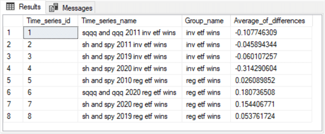
Here is the results set from the preceding script.

The time series with time_series_id values of 1 through 4 belong to the inv ETF wins group. All the time series belonging to this group have negative average_of_differences values.
The time series with time_series_id values of 5 through 8 belong to the reg ETF wins group. All the time series belonging to this group have positive average_of_differences values.

Compute an inter-object distance matrix

The next step is to compute a distance matrix between the objects in a set.

The code listing below is an excerpt from the script to compute the Euclidean distances between the time series objects.

The script starts by declaring and populating a collection local variable values based on the Average_of_differences for each time series object. These differences represent the location of each time series object on a single dimension.
Next, the code drops any prior version of the inter_time_series_object_Euclidean_distance_matrix table. This table persists the pairwise Euclidean distances between objects.
Then, a select statement computes Euclidean distances between time series objects based on the local variable values.
- The complete code listing, of which only an excerpt shows below, consists of eight selected statements nested in an outer select statement. Each of the eight nested select statements generates a results set comprised of a single row. The results for each nested selected statement are concatenated into a single results set by union operators.
- The columns in the first row compute the distances of the first time series object to every time series in the set of eight time series.
  - A power function for each column squares the average of the differences between the first time series and each of the other time series, including the first time series.
  - A sqrt function computes the square root of the squared value.
  - These two expressions for each column in the row implement the Euclidean function for the distance between two objects represented by values on a single dimension.
- An ellipsis sign denotes the omitted code for computing the distances to time series id values 3 through 7.
- An into statement just before the from clause in the outer select statement inserts the Euclidean distances between all pairs of time series objects into the inter_time_series_object_Euclidean_distance_matrix table.
The script below concludes with a select statement that displays the Euclidean distances in the inter_time_series_object_Euclidean_distance_matrix table.

-- compute the distance matrix between the time series objects
 
-- declare local variables for the average difference between regular etfs less inverse etfs
-- for each time series object
declare 
 @time_series_1_average_difference float =(select Average_of_differences from dbo.reg_and_inverse_etfs_for_knn where Time_series_id = 1)
,@time_series_2_average_difference float =(select Average_of_differences from dbo.reg_and_inverse_etfs_for_knn where Time_series_id = 2)
,@time_series_3_average_difference float =(select Average_of_differences from dbo.reg_and_inverse_etfs_for_knn where Time_series_id = 3)
,@time_series_4_average_difference float =(select Average_of_differences from dbo.reg_and_inverse_etfs_for_knn where Time_series_id = 4)
,@time_series_5_average_difference float =(select Average_of_differences from dbo.reg_and_inverse_etfs_for_knn where Time_series_id = 5)
,@time_series_6_average_difference float =(select Average_of_differences from dbo.reg_and_inverse_etfs_for_knn where Time_series_id = 6)
,@time_series_7_average_difference float =(select Average_of_differences from dbo.reg_and_inverse_etfs_for_knn where Time_series_id = 7)
,@time_series_8_average_difference float =(select Average_of_differences from dbo.reg_and_inverse_etfs_for_knn where Time_series_id = 8)
 
-- Remove prior inter_time_series_object_Euclidean_distance_matrix
if exists(select * from  sys.objects where name  = 'inter_time_series_object_Euclidean_distance_matrix' and TYPE =  'u')
    DROP TABLE  dbo.inter_time_series_object_Euclidean_distance_matrix
 
-- use the local variables to compute a Euclidean distance matrix between the time series objects
-- based on the local variables with the average difference between regular and inverse etfs
-- for each time series object
select *
into inter_time_series_object_Euclidean_distance_matrix
from
(
select 
  1 Time_series_id
, sqrt(power(@time_series_1_average_difference - @time_series_1_average_difference,2)) [distance from time_series_1]
, sqrt(power(@time_series_1_average_difference - @time_series_2_average_difference,2)) [distance from time_series_2] 
, sqrt(power(@time_series_1_average_difference - @time_series_3_average_difference,2)) [distance from time_series_3] 
, sqrt(power(@time_series_1_average_difference - @time_series_4_average_difference,2)) [distance from time_series_4] 
, sqrt(power(@time_series_1_average_difference - @time_series_5_average_difference,2)) [distance from time_series_5] 
, sqrt(power(@time_series_1_average_difference - @time_series_6_average_difference,2)) [distance from time_series_6] 
,sqrt(power( @time_series_1_average_difference - @time_series_7_average_difference,2)) [distance from time_series_7] 
,sqrt(power( @time_series_1_average_difference - @time_series_8_average_difference,2)) [distance from time_series_8] 
union
select
  2 Time_series_id
, sqrt(power(@time_series_2_average_difference - @time_series_1_average_difference,2)) [distance from time_series_1]
, sqrt(power(@time_series_2_average_difference - @time_series_2_average_difference,2)) [distance from time_series_2] 
, sqrt(power(@time_series_2_average_difference - @time_series_3_average_difference,2)) [distance from time_series_3] 
, sqrt(power(@time_series_2_average_difference - @time_series_4_average_difference,2)) [distance from time_series_4] 
, sqrt(power(@time_series_2_average_difference - @time_series_5_average_difference,2)) [distance from time_series_5] 
, sqrt(power(@time_series_2_average_difference - @time_series_6_average_difference,2)) [distance from time_series_6] 
,sqrt(power( @time_series_2_average_difference - @time_series_7_average_difference,2)) [distance from time_series_7] 
,sqrt(power( @time_series_2_average_difference - @time_series_8_average_difference,2)) [distance from time_series_8] 
union
.
.
.
 
union
select
  8 Time_series_id
, sqrt(power(@time_series_8_average_difference - @time_series_1_average_difference,2)) [distance from time_series_1]
, sqrt(power(@time_series_8_average_difference - @time_series_2_average_difference,2)) [distance from time_series_2] 
, sqrt(power(@time_series_8_average_difference - @time_series_3_average_difference,2)) [distance from time_series_3] 
, sqrt(power(@time_series_8_average_difference - @time_series_4_average_difference,2)) [distance from time_series_4] 
, sqrt(power(@time_series_8_average_difference - @time_series_5_average_difference,2)) [distance from time_series_5] 
, sqrt(power(@time_series_8_average_difference - @time_series_6_average_difference,2)) [distance from time_series_6] 
,sqrt(power( @time_series_8_average_difference - @time_series_7_average_difference,2)) [distance from time_series_7] 
,sqrt(power( @time_series_8_average_difference - @time_series_8_average_difference,2)) [distance from time_series_8] 
) for_distance_matrix
 
-- display the inter_time_series_object_Euclidean_distance_matrix
select * from dbo.inter_time_series_object_Euclidean_distance_matrix

The Euclidean distance matrix from the preceding script appears in the next screen shot.

The first column contains a sequence of integer values for 1 through 8. Each row in the column denotes a distinct time series object by its time_series_id value.
The column names for each of the remaining columns reference the pairwise distances from each object to each other object.
- For example, the first numerical value in the second column is 0 because the distance between time series 1 and itself is 0.
- The numerical value in the second column is 0.061851965. This is the outcome of the Euclidean distance function for time series 1 and time series 2.
- Notice that all diagonal values for columns two through nine have 0 values because these cells compute the distance between an object and itself.
  - If you examine the pairwise distances between objects, you can recognize that the values in the distance matrix are symmetric around the diagonal values. This is because Euclidean distances do not depend on the order of the objects.
  - Therefore, the distance between time series 1 and time series 2 (0.061851965) is the same as distance between time series 2 and time series 1 (0.061851965).

Displaying computed group assignments based on K equals 1

The purpose for computing the inter-object distance matrix is to find the K nearest neighbors to each object, and then assign the most common group from among the nearest neighbors. When K equals 1, then there is just 1 nearest neighbor. As a result, the group for the nearest neighbor becomes the assigned group for an object.

Here is an excerpt from the script to derive assigned groups for objects based on the group for a nearest neighbor to an object.

The full script has eight select statements whose results sets are concatenated by union operators into single results set.
The following excerpt from the full script shows the code for the first, second, and eighth time series objects.
Each block of code for an object consists of an inner query embedded in an outer query.
- The inner query returns the top row whose distance is not zero from the inter-object distance matrix. This code returns the time series id value for the nearest neighbor to the object.
- The outer query returns the time series id value for the object to which you want to assign a group, the time_series_id value for the nearest neighbor, and the group name that you want to assign.
The ellipsis after the second object and before the eighth object is where the code for the third through the seventh time series objects go.
The code for the eighth time series object is the last object in the excerpt.

-- KNN time series classifications for K = 1
 
-- Time_series_1 is nearest to the following
-- Time_series_id in Group_name
select 'Time_series_id = 1' [source time series], Time_series_id [nearest time_series_id], Group_name from dbo.reg_and_inverse_etfs_for_knn
where Time_series_id =
(
select top 1
 Time_series_id --, [distance from time_series_1] 
from dbo.inter_time_series_object_Euclidean_distance_matrix
where [distance from time_series_1] <> 0
order by [distance from time_series_1] 
)
 
union
  
-- Time_series_2 is nearest to the following
-- Time_series_id in Group_name
select 'Time_series_id = 2' [source time series], Time_series_id [nearest time_series_id], Group_name from dbo.reg_and_inverse_etfs_for_knn
where Time_series_id =
(
select top 1
 Time_series_id --, [distance from time_series_1] 
from dbo.inter_time_series_object_Euclidean_distance_matrix
where [distance from time_series_2] <> 0
order by [distance from time_series_2] 
)
 
union
 
.
.
.
 
union
 
 
-- Time_series_8 is nearest to the following
-- Time_series_id in Group_name
select 'Time_series_id = 8' [source time series], Time_series_id [nearest time_series_id], Group_name from dbo.reg_and_inverse_etfs_for_knn
where Time_series_id =
(
select top 1
 Time_series_id --, [distance from time_series_1] 
from dbo.inter_time_series_object_Euclidean_distance_matrix
where [distance from time_series_8] <> 0
order by [distance from time_series_8] 
)

Here is the result set from the complete version of the preceding script.

The first column denotes the time series to which a group name is to be assigned. The Group_name column returns the assigned group name for the object specified in the first column.
As you can see,
- The first four time series are assigned a group name of inv ETF wins.
- The second four time series are assigned a group name of reg ETF wins.
- You can confirm the assignments for the first four time series and the second four time series by referring to the original source data in the "Insert the objects in a table for computing inter-object distances" section.

Displaying computed group assignments based on K equals 3

When K is greater than 1, then T-SQL codes more functionality than when you are searching for the group to which the single nearest neighbor resides.

First, the code needs to find the K nearest neighbors with the group names to which the neighbors belong.
Second, the code needs to find the groups to which the K nearest neighbors belong.
Third, the code needs to pick the group to which the majority of K nearest neighbors belong. In order to assure that there is a majority group among the K nearest neighbors, you need to pick a K value for which there will always be a majority winner. In the case of just two groups (as in this tip), a K value of 3 is the first K value that ensures an odd number of groups in a way that lets you derive a majority group winner.

The following script shows how to derive the three nearest neighbors to time series 1.

The script includes a derived table named for_K_nearest. The query for the derived table returns the time_series_id values for each of the three closest neighbors to time series 1.
An outer query joins the results set from the for_K_nearest derived table to a query whose source is the reg_and_inverse_etfs_for_knn table. Recall that reg_and_inverse_etfs_for_knn table includes a separate row for each time series, as well as the group for each time series and selected other source data.

-- Time series 1 is nearest to the three following
-- Time_series_ids in the Group_name values
select 
 'Time_series_id = 1' [source time series]
,dbo.reg_and_inverse_etfs_for_knn.Time_series_id [nearest time_series_id]
,Group_name 
from dbo.reg_and_inverse_etfs_for_knn
 
inner join
 
(
select top 3
 Time_series_id 
from dbo.inter_time_series_object_Euclidean_distance_matrix
where [distance from time_series_1] <> 0
order by [distance from time_series_1] 
) for_K_nearest
 
on dbo.reg_and_inverse_etfs_for_knn.Time_series_id = for_K_nearest.Time_series_id

Here is what the output from the preceding query looks like. The results set from the script includes three columns.

The source time series column designates the name of the time series for which the script finds the 3 closest time series based on the Euclidean distance matrix between objects. To keep the example easy to follow, the source time series column value is hard coded in the script above. This example code is for the 3 nearest neighbors to the first time series.
The second column displays the time_series_id value for each of the 3 nearest time series to time series 1.
TThe third column shows the Group_name value for each of the 3 nearest neighbors. Two of these neighbors belong to the inv ETF wins group. Therefore, that's the majority wins group for time series 1.

It is possible to adapt the preceding script to pick automatically the majority wins group for time series 1. The following screen shot shows the adapted script with the code to pick the majority group winner highlighted in yellow.

A new outer query is added.
The select statement for the outer query has list items for showing the source time series id value, which is 1 in the following example, the majority winner Group_name value, and the number of neighbors comprising the majority.
The highlighted code towards the bottom of the script
- Inner joins the results set from the preceding query to the original source data in the reg_and_inverse_etfs_for_knn table
- Then, a group by clause with a having clause criterion selects the Group_name occurring the majority number of times

Here is what the output looks like. The group by clause with its having criterion causes the query to return a single row with the Group_name value for the majority of the nearest neighbors as well as the number of neighbors in the majority.

You can concatenate a series of updated scripts like the one above for each of the remaining seven time series in this tip. Follow each updated script with a union operator for each additional time series. The complete version of this script for the full set of time series is included in the download for this tip. The output from the complete version of the script appears below.

As you can see, there is a separate row for each source time series.
The first four time series are all assigned to the inv ETF wins group.
Three of the second set of four etfs are assigned to the reg ETF wins group.
The Group_name value for the fifth time series is incorrectly assigned to the inv ETF wins group. However, you can verify from the display of the input source data that the correct assigned group for the fifth time series should be reg ETF wins and not inv ETF wins.
Therefore, the assigned Group_name values are less valid for a K of 3 than for a K of 1.

Next Steps

This tip targets anyone with a basic understanding of T-SQL and an interest in knowing more about the KNN algorithm for grouping objects. There are two files in the download for this tip.

One of the download files contains the source time series data. The data are available in an .xlsx file.
The download file contains the T-SQL code for applying the KNN algorithm as discussed in this tip.

The KNN algorithm is a very commonly used data science algorithm for grouping objects based on their position in a coordinate space. Here are two additional references for you to get started learning more about the algorithm.

About the author

Rick Dobson is an author and an individual trader. He is also a SQL Server professional with decades of T-SQL experience that includes authoring books, running a national seminar practice, working for businesses on finance and healthcare development projects, and serving as a regular contributor to MSSQLTips.com. He has been growing his Python skills for more than the past half decade -- especially for data visualization and ETL tasks with JSON and CSV files. His most recent professional passions include financial time series data and analyses, AI models, and statistics. He believes the proper application of these skills can help traders and investors to make more profitable decisions.

This author pledges the content of this article is based on professional experience and not AI generated.

View all my tips

Implement K Nearest Neighbor Solution with T-SQL