Contingency Table Analysis via Chi Square using T-SQL: Part 1

By: Rick Dobson   |   Comments (2)   |   Related: > TSQL

Problem

Please provide an introduction for how to analyze contingency tables with SQL. Demonstrate how to derive contingency tables from a simple dataset. Also, provide a SQL framework for analyzing a contingency table via the Chi Square test statistic.

Solution

Do you want to leverage your dataset and SQL scripting skills for data science projects? Well, this tip is one place for you to start doing just that. An article on the DataCamp website motivated this tip; the DataCamp website is a tutorial and training resource for data science development skills. The article featured an introduction to contingency tables using the popular R language with the Chi Square test and other statistical tools. This tip aims to illustrate how you can create contingency tables and analyze them with a SQL script and the Chi Square test. A major goal of the tip is to illustrate one way to leverage SQL scripting in a typical data science project.

Both R and Python scripting environments feature much built-in functionality to facilitate data science projects, but they are not especially well endowed with relational database management features. On the other hand, SQL, as implemented by Microsoft with SQL Server and other leading SQL database providers, offers outstanding data management features and basic scripting capabilities that can be applied within data science projects. Using SQL instead of R or Python can make sense – especially when the data for a project are already stored (or destined to be stored) in a SQL database.

In this tip, you will see how to use a classic data science source (here and here) and SQL Server scripting features in a data science project. In addition to using a classic data science source, this tip also compares SQL and R for performing multiple steps in a data science project from accessing a dataset, to performing exploratory data analysis, to computing a contingency table, to computing a Chi Square statistic.

What is a contingency table?

Within statistics, a contingency table represents counts for two or more distinct sets of random discrete variables. The Data Science with SQL Server for Inferential and Predictive Statistics: Part 2 tip illustrates the layout of a two-way contingency table in a format suitable for analysis with SQL scripting. For your easy reference, the layout also appears below. This tip demonstrates computational and statistical techniques for a two-way contingency table.

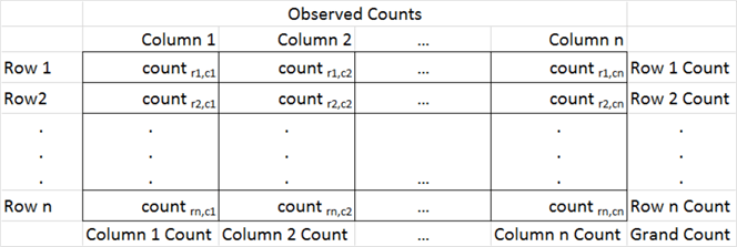
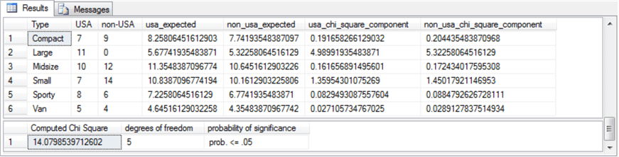
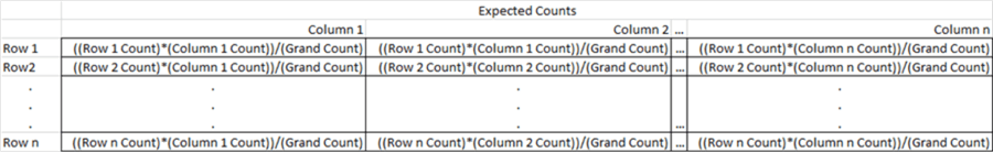
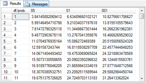
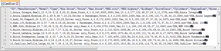
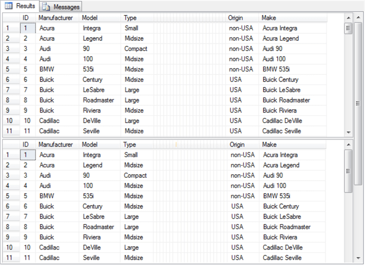
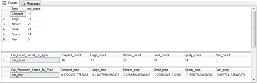
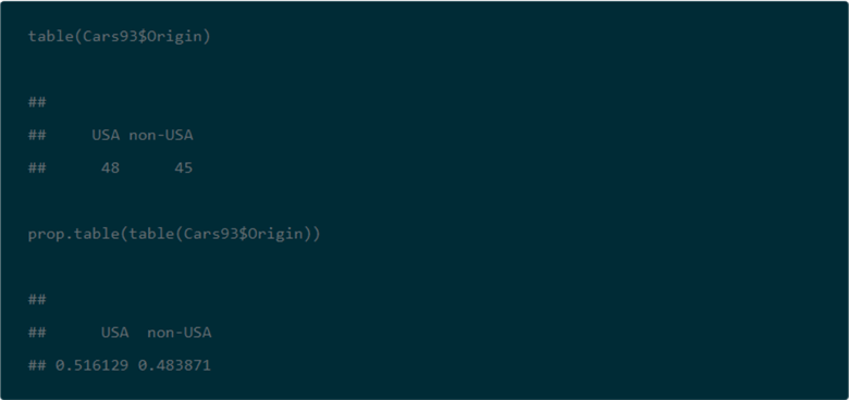
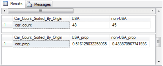
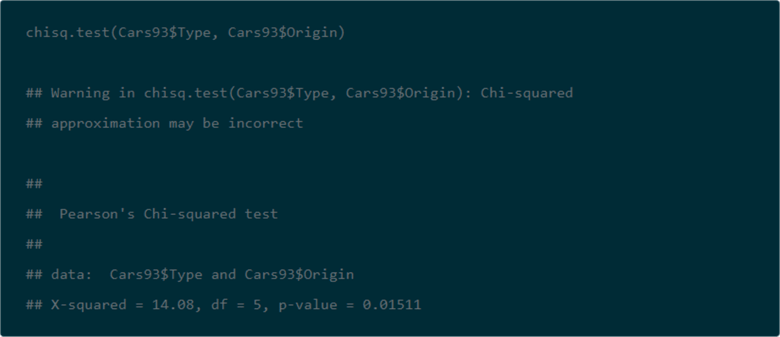
The contingency table consist of the cells with counts in them; the table normally appears with row and column labels. The row of column label values with Column 1 through Column n denote one set of discrete variables. The row label values with Row 1 through Row n denote a second set of discrete variables. Notice that each cell with a count in it also has two subscripts, such as count _r1,c1 and count _rn,cn; these cells represent the count or frequency of observations at the intersection of column category variables and row category variables. The number of columns does not have to equal the number of rows so, for example, a contingency table could have n rows and m columns where n is not equal to m.

There are three additional sets of values that are not strictly part of the contingency table. There is a row of column footers labeled Column 1 Count through Column n Count. These represent the sum of count values, respectively, in columns 1 through n. Similarly, there is a column of values to the right of the contingency label with the values Row 1 Count through Row n Count. These represent the sum of count values, respectively, in rows 1 through n. There is a third set consisting of just one additional value with the label Grand Count, which is the sum of all count values across all rows and columns. These three additional sets of values to the bottom and right of the contingency table are frequently useful for calculating expected values. By comparing the observed counts to the expected counts with a Chi Square statistic, you can assess the independence of the column category variable values from the row category variable values.

What is a Chi Square test for a contingency table?

There are two types of Chi Square tests for contingency tables.

• One test is called a Chi Square test for independence. This kind of test assesses the degree of association between row and column category variables for a single population.
• The other test is called a Chi Square test for homogeneity. This kind of test assesses if a set of category variable proportions are the same across two or more different populations.

The Data Science with SQL Server for Inferential and Predictive Statistics: Part 2 tip includes a layout for computing expected values based on the independence of row and column category variables. This layout is duplicated below for your easy reference. As you can see, the expected value for a cell is the product of the row sum for a cell and the column sum for a cell divided by the grand count across all cells. Notice that cells in the following table of expected values have the same layout as the observed values in the contingency table.

• For example, the ((Row 1 Count)*(Column 1 Count))/(Grand Count) expression for the cell at the intersection of Row 1 and Column 1 in the screen shot below is the expected value for the corresponding observed value with a value of count _r1,c1 in the preceding screen shot.
• In like manner, the ((Row n Count)*(Column n Count))/(Grand Count) expression for the cell at the intersection of Row n and Column n in the screen shot below is the expected value for the corresponding observed value with a value of count _rn,cn in the preceding screen shot.

Even though the sampling plan (or how you collect data) for each kind of test is different, the computational details are the same for both the test for independence and the test for homogeneity. There is a restriction regarding the count per cell that is variously expressed in different sources (here, here, and here). For example, it is sometimes indicated that the minimum observed count must not be less than five. Other sources indicate that no more than twenty percent of the expected counts can be less than five. This tip does not take a position about the count per cell. If your contingency table does not conform to a set of minimum requirements or you cannot re-group the categorical data to conform to a set minimum count requirements, then you can consider another type of test instead of the Chi Square test.

The computed Chi Square value is based on the squared difference between each cell's observed and expected values divided by the cell's expected value summed across all cells in the contingency table. Wikipedia demonstrates the application of this approach to calculating a computed Chi Square value for categorical data from a contingency table in the "Example chi-squared test for categorical data" section of its Chi-squared test page.

In order to use the computed Chi Square value for either of the two Chi Square contingency tests, you need to compare the computed Chi Square value to a corresponding critical Chi Square value at an appropriate statistical significance level. Critical Chi Square values are defined by two parameters: the number of degrees of freedom and a level of statistical significance. The degrees of freedom for a two-way contingency table is the number of rows less one multiplied by the number columns less one. The most common statistical significance levels are the .05, .01, and .001; these are the statistical significance levels used in this tip.

The critical Chi Square values for any degrees of freedom and statistical probability level can be derived from Excel's CHISQ.INV.RT function. MSSQLTips.com has multiple tips describing how to populate a SQL Server table of critical Chi Square values from the CHISQ.INV.RT function (for example, see the "Introduction to Goodness-of-fit Chi Square test" section in the Using T-SQL to Assess Goodness of Fit to an Exponential Distribution tip).

The table of critical Chi Square values for this tip resides in the Chi Square Critical Values 05 01 001 table of the AllNasdaqTickerPricesfrom2014into2017 database. The table is populated from an Excel worksheet with CHISQ.INV.RT function values imported into the SQL Server table. You can import the Excel worksheet, which is available as a download with this tip, to populate a SQL Server table in any database of your choice. The following screen shot shows an excerpt from the full table. The excerpt shows that critical Chi Square values increase with increasing degrees of freedom and statistical probability levels that are progressively rarer.

• The first column (df/prob.) denotes the degrees of freedom for critical Chi Square values.
• The second, third, and fourth columns have names of 05, 01, and 001 for the .05, .01, and .001 statistical probability levels. Among the three levels, the .05 level is the least rare level, and the .001 is the rarest level.
• The full table includes critical Chi Square values for degrees of freedom values from one through one hundred fifty.

The null hypothesis for the Chi Square test is that there is no difference between the set of observed counts and the set of expected counts. If the computed Chi Square value exceeds a critical Chi Square value at a given probability level, then the null hypothesis is statistically rejected at that probability.

• For example, if you were testing a contingency table for independence between row and column categorical variables, and the computed Chi Square value was less than the critical Chi Square value, then you would accept the null hypothesis of row and column categorical variable independence.
• On the other hand, if you were testing a contingency table for homogeneity of response across groups and the computed Chi Square value was greater than or equal to the critical Chi Square value at a statistical probability level, then you could reject the null hypothesis of homogeneity of response across populations.

The data for the contingency table

This tip uses the Cars93 dataset that ships with the R programming language package. This dataset has one row per make (comprised of a manufacturer and a model) with a top row of field names. This dataset is available from numerous sources; this tip demonstrates how to import the dataset into SQL Server from this source. When you click a link labeled "download this file" from the source, a csv file downloads to your computer, but the file has a non-standard format relative to typical Windows csv files. The following screen shot shows an excerpt from a Notepad++ session with the file after some minor editing. The editing removed double quote marks around field values in lines 2 through 94 and added ID as the first field name to line 1.

• Line 1 contains field names.
• Lines 2 through 94 contain field values.
• There are three main types of values:
  • String values with alphabetic characters, such as Acura, Audi, BMW, and Buick.
  • Numbers in an integer format, such as 31, 25, and 26
  • Numbers with a decimal point, such as 12.9, 29.2, and 25.9

The field and row terminators are, respectively, comma (,) and linefeed (LF). While the comma is a typical for a Windows csv file, the LF terminator is not typical. In fact, this formatting convention is typical for csv files in Unix and Linux operating systems. A prior tip demonstrates the need to use a special rowterminator code ('0x0a') in SQL Server when importing csv files terminating in LF.

The following SQL script uses a two-step process for importing the Cars93.csv file into a SQL Server table. In the first step, all fields, except for ID, are imported as variable length character fields with a varchar (50) specification. The ID field is a number identifier for rows in the file, and its values are imported with an int data type. In the second step, the number field values, except for ID, are converted to int or float depending on whether they contain, respectively, integer data or data with a decimal point. The script additionally demonstrates some other features for importing data science datasets into SQL Server that you may find useful.

• The script starts by creating a fresh copy of the #temp local temporary table. The field names correspond to the fields denoted in the first line of the Cars93.csv file.
• Next, a bulk insert command transfers data rows from the Cars93.csv file to the #temp table.
  • The from file is stored in the c:\for_statistics path. You can change this to any other path in which you have saved a from file for import to SQL Server.
  • The rowterminator field value is designated as '0x0a', which represents the LF at the end of data rows.
• After the data are initially imported into the #temp table in SQL Server, they are transformed and cleaned in various ways to represent their true value. The cleaned values are stored in a second local temporary table named #temp_clean; a fresh copy of the #temp_clean data type is prepared before the cleaning. This process comprises the second step for importing data to SQL Server.
  • All string fields are imported as captured by the varchar (50) data type.
  • The ID field is left in its int format.
  • Number values with a decimal point are converted to a float data type with the exception of number column values denoted as NA for missing data.
  • Number values without a decimal point are converted to an int data type with the exception of number column values denoted as NA for missing data.
  • Number fields with an NA value for missing values are imported as a NULL SQL Server value.
  • The Cylinders column is saved with an int data type except for rows with a value of ‘rotary'; this is because rotary engines do not have fixed cylinders. Rotary, for rotary engine, essentially denotes a NULL SQL Server value for the Cylinders column.

-- create fresh copy of #temp with varchar fields
-- except for ID int column
begin try
drop table #temp
end try
begin catch
print '#temp not available to drop'
end catch
  
create table #temp(
 ID INT
,Manufacturer varchar(50)
,Model varchar(50)
,Type varchar(50)
,"Min.Price" varchar(50)
,"Price" varchar(50)
,"Max.Price" varchar(50)
,"MPG.city" varchar(50)
,"MPG.highway" varchar(50)
,"AirBags" varchar(50)
,"DriveTrain" varchar(50)
,"Cylinders" varchar(50)
,"EngineSize" varchar(50)
,"Horsepower" varchar(50)
,"RPM" varchar(50)
,"Rev.per.mile" varchar(50)
,"Man.trans.avail" varchar(50)
,"Fuel.tank.capacity" varchar(50)
,"Passengers" varchar(50)
,"Length" varchar(50)
,"Wheelbase" varchar(50)
,"Width" varchar(50)
,"Turn.circle" varchar(50)
,"Rear.seat.room" varchar(50)
,"Luggage.room" varchar(50)
,"Weight" varchar(50)
,"Origin" varchar(50)
,"Make" varchar(50)
)
  
-- cars93.csv is download from:
-- https://forge.scilab.org/index.php/p/rdataset/source/tree/master/csv/MASS/Cars93.csv
 
-- manual modifications to downloaded csv file
-- convert first column designator from "" to "ID" in first row
-- remove double-quote delimiters for column values in second through ninety-fourth rows
 
-- from file rows terminate with line feed character only as in Unix and Linux
-- so rowterminator is set to '0x0a' 
 
bulk insert #temp
        from 'C:\for_statistics\cars93.csv'
        with
       (
          firstrow = 2
         ,fieldterminator = ','
         ,rowterminator = '0x0a' 
        )
go
  
-- create fresh copy of #temp_clean
begin try
drop table #temp_clean
end try
begin catch
print '#temp_clean not available to drop'
end catch 
 
-- cleaned #temp table into #temp_clean with
-- int and float assignments for fields with numbers
-- text catches for NA and rotary in 
-- Cylinders, [Rear.seat.room], [Luggage.room] columns
select 
 ID
,Manufacturer
,Model
,Type
,cast([Min.Price] as float) [Min.Price]
,cast(Price as float) Price
,cast([Max.Price] as float) [Max.Price]
,cast([MPG.city] as int) [MPG.city]
,cast([MPG.highway] as int) [MPG.highway]
,AirBags
,DriveTrain
,
 case
   when [Cylinders] = 'rotary' then NULL
   else cast([Cylinders] as int)
 end [Cylinders]
,cast(EngineSize as float) EngineSize
,cast(Horsepower as int) Horsepower
,cast(RPM as int) RPM
,cast([Rev.per.mile] as int) [Rev.per.mile]
,[Man.trans.avail]
,cast([Fuel.tank.capacity] as float) [Fuel.tank.capacity]
,cast(Passengers as int) Passengers
,cast(Length as int) Length
,cast(Wheelbase as int) Wheelbase
,cast(Width as int) Width
,cast([Turn.circle] as int) [Turn.circle]
,
 case
   when [Rear.seat.room] = 'NA' then NULL
   else cast([Rear.seat.room] as float)
 end [Rear.seat.room]
,
 case
   when [Luggage.room] = 'NA' then NULL
   else cast([Luggage.room] as int)
 end [Luggage.room]
,cast(Weight as int) Weight
,Origin
,Make
 
into #temp_clean
from #temp
 
-- echo original source data and cleaned data
-- primarily for clarifying input data processing
select * from #temp
select * from #temp_clean
			

The last two lines in preceding script display the contents of the #temp and #temp_clean tables. These statements are not strictly necessary, but it is often useful to echo data after the completion of critical steps. The next screen shot contains excerpts from the #temp and #temp_clean tables.

• The top pane shows data from the #temp table.
• The bottom pane shows data from the #temp_clean table.
• Additionally, select columns are compressed so they do not display in order to display just critical columns that will be highlighted later in this tip.
  • Type and Origin are critical because these columns appear in a contingency table based on the Cars93.csv file.
  • Manufacturer, Model, and Make are critical in identifying the car to which a row in the dataset refers.

SQL versus R for exploratory data analysis

The DataCamp tutorial on contingency tables with R starts with some exploratory data analysis. Many data scientists will begin the analysis of a dataset with some exploratory data analysis to become familiar with the data source that they plan to mine and/or model in subsequent processing steps. After a simple listing of values in the database in a way that is similar to the preceding screen shot, the tutorial reports some exploratory data analysis for key fields. For example, the following screen shot from the tutorial shows the syntax and results for tabulated counts and proportions by Type from the Cars93 dataset. The top portion of the screen shot is for car count by Type, and the bottom portion of the screen shot is for car proportion by Type.

• The R syntax is very compact for this way of displaying data.
  • The top portion of the screen shot shows a single line of code is required to generate a horizontal display of the counts by type.
    • The source dataset is Cars93.
    • The column to be tabulated has the name Type.
    • The table function generates the count of cars by Type.
  • The bottom portion of the screen shot illustrates the R syntax for the prop function to calculate and report the proportions by Type.
    • The source data is again the Type data in Cars93.
    • The table function computes count by Type for the source data.
    • The prop function computes proportions by Type from count by Type.

The following code segment displays SQL syntax for arriving at comparable results. The SQL code is less compact than the R code for at least a couple of reasons. SQL is not optimized for exploratory data analysis, and it is more natural with SQL to display results vertically rather than horizontally.

• The declare statement at the top of the script defines the @all_cars variable as the count of all rows in the #temp_clean table. Recall that this table is based, after some cleaning, on the Cars93 dataset. Other variable declarations are defined for a portion of the script outside of code that displays below.
• Next, the #temp_car_count_by_type local temporary table is defined, populated and displayed; this table contains the count of cars by Type. Results are displayed vertically instead of horizontally as in the R script output.
• Therefore, the results in the #temp_car_count_by_type table are pivoted with the pivot operator so that SQL can display results horizontally as in the preceding script. You can find an introduction to the pivot operator in this prior tip. Notice that the script for pivoting has the #temp_car_count_by_type table as its source.
• The last portion of the SQL script computes the proportion of car count by type. This segment of the code also uses the pivot operator, and the code additionally depends on the #temp_car_count_by_type table. However, the @all_cars variable is used to define proportion by Type.

-- declare/populate local variables for storing intermediate
-- scalar values for reuse in script
declare 
 @all_cars float =(select count(*) from #temp_clean)
,@computed_chi_square float
,@df int
,@05 float
,@01 float
,@001 float
 
-- create fresh copy of #temp_car_count_by_type
begin try
drop table #temp_car_count_by_type
end try
begin catch
print '#temp_car_count_by_type not available to drop'
end catch
 
-- this is for a source table in a pivot query
-- it is referenced by #temp_car_count_by_type in the pivot query
-- it is derived from a #temp_clean
select Type, count(ID) AS car_count   
into #temp_car_count_by_type
FROM #temp_clean 
group by Type;
 
-- echo #temp_car_count_by_type
   select * from #temp_car_count_by_type
 
-- pivot table with one row and six column counts  
select 
 'car_count' Car_Count_Sorted_By_Type   
,[Compact] Compact_count
,[Large] Large_count
,[Midsize] Midsize_count
,[Small] Small_count
,[Sporty] Sporty_count
,[Van] Van_count
from  
(select Type, car_count from #temp_car_count_by_type) AS SourceTable  
pivot  
(  
avg(car_count) -- avg function captures previously aggregated value in SourceTable
FOR Type IN([Compact], [Large], [Midsize], [Small], [Sporty], [Van])  
) AS PivotTable; 
 
-- pivot table with one row and six column proportions  
SELECT 'car_prop' Car_Proportion_Sorted_By_Type,   
 [Compact]/@all_cars [Compact_prop]
,[Large]/@all_cars [Large_prop]
,[Midsize]/@all_cars [Midsize_prop]
,[Small]/@all_cars [Small_prop]
,[Sporty]/@all_cars [Sporty_prop]
,[Van]/@all_cars [Van_prop]
FROM  
(select Type, car_count from #temp_car_count_by_type) AS SourceTable  
pivot  
(  
avg(car_count) -- avg function captures previously aggregated value in SourceTable
FOR Type IN([Compact], [Large], [Midsize], [Small], [Sporty], [Van])  
) pivotable; 
			

Here's the output from the preceding SQL script.

• The #temp_car_count_by_type local temporary table appears initially. Its results display vertically.
• Next, the pivoted version of the #temp_car_count_by_type local temporary table appears. In this case, the results appear horizontally. These results from SQL exactly match those from R in the preceding screen shot.
• The next horizontal data display is for the proportion of cars by type. The SQL code displays its results to more places of accuracy, but its results are otherwise the same as those from R.

The DataCamp tutorial next directs its attention to counts and proportions for cars by Origin. Cars are classified as manufactured in the USA or in a non-USA country. The reason for exploring this second variable is that its categories will eventually be used in a contingency table as well as a Chi Square test. The code is very compact and follows the same convention as for the car counts and proportions presented above.

The next code excerpt is for computing car count and proportion by Origin from a SQL script. The approach follows the same general design as for car count and proportion by Type with the exception that for this script the aggregation of car count by Origin in a vertical alignment is not displayed. However, the aggregation of car count by Origin in a horizontal alignment is generated and displayed in the script below. Because this script is designed to be run immediately after the preceding script, there is no need to declare and populate the @all_cars variable.

-- create fresh copy of #temp_car_count_by_origin
begin try
drop table #temp_car_count_by_origin
end try
begin catch
print '#temp_car_count_by_origin not available to drop'
end catch
  
-- source table name is #temp_car_count_by_origin
-- it is derived from a #temp_clean
select Origin, count(ID) AS car_count   
into #temp_car_count_by_origin
from #temp_clean 
group by Origin;
 
-- create fresh copy of #temp_car_count_by_origin
begin try
drop table #temp_pivoted_car_count_by_origin
end try
begin catch
print '#temp_pivoted_car_count_by_origin not available to drop'
end catch
 
-- pivot table with one row and two column counts  
select 'car_count' Car_Count_Sorted_By_Origin,   
[USA], [non-USA]
into #temp_pivoted_car_count_by_origin
from  
(select Origin, car_count from #temp_car_count_by_origin) AS SourceTable  
pivot  
(  
avg(car_count) -- avg function captures previously aggregated value in SourceTable
FOR Origin IN([USA], [non-USA])  
) pivottable; 
 
select * from #temp_pivoted_car_count_by_origin
 
-- pivot table with one row and two column counts  
select 'car_prop' Car_Count_Sorted_By_Origin,   
[USA]/@all_cars [USA_prop], [non-USA]/@all_cars [non-USA_prop]
from  
(select Origin, car_count from #temp_car_count_by_origin) AS SourceTable  
pivot  
(  
avg(car_count) -- avg function captures previously aggregated value in SourceTable
FOR Origin IN([USA], [non-USA])  
) pivottable;  
			

Here's the output from the preceding SQL script. Again, the SQL results match the R results, except for the number of places to which values are rounded.

SQL versus R for contingency table calculation

The next screen shot shows the R script and its result for computing a contingency table from the Type and Origin in the Cars93 dataset. This script saves the contingency table to the tab1 object. As you will see later when we are computing a Chi Square test, it is not strictly necessary to save the contingency table in order to use it again.

The next SQL script excerpt illustrates one approach to computing a contingency table for the Type and Origin in the Cars93 dataset.

• This approach begins by creating a subset of the Cars93 data from the #temp_clean table.
  • The name of the subset is #temp_row_id_by_col_id_ID.
  • This subset table is populated by three columns from the #temp_clean table:
    • ID
    • Origin
    • Type
  • Because the subset table contains all rows, it consists of ninety-three rows, which is the full set of rows from #temp_clean and ultimately the Cars93 dataset.
• Next, the pivot operator and an aggregate function (namely, count) compute the contingency table from the #temp_clean subset.
  • Within the pivot operator, a count function aggregates cars by Origin (USA and non-USA) in the #temp_clean subset. The Origin values become the columns of the contingency table.
  • Then, the outer query invoking the pivot operator, joins Type to the query result set. The Type values become the rows of the contingency table.
  • The contingency table is saved with the into keyword to the #temp_type_by_origin_car_count table.
• Finally, a select statement displays the contingency table in #temp_type_by_origin_car_count.

-- create fresh copy of #temp_row_id_by_col_id_ID
begin try
drop table #temp_row_id_by_col_id_ID
end try
begin catch
print '#temp_row_id_by_col_id_ID not available to drop'
end catch
  
-- source table name is #temp_type_by_car_count
-- it is derived from a #temp_clean
SELECT ID, Origin, Type   
into #temp_row_id_by_col_id_ID
FROM #temp_clean 
 
-- echo of #temp_row_id_by_col_id_ID
select * from #temp_row_id_by_col_id_ID
 
-- create fresh copy of #temp_type_by_origin_car_count
begin try
drop table #temp_type_by_origin_car_count
end try
begin catch
print '#temp_type_by_origin_car_count not available to drop'
end catch
 
-- This is the contingency table
select Type, [USA], [non-USA]
into #temp_type_by_origin_car_count
from 
(select Type, Origin, ID  
from #temp_row_id_by_col_id_ID) p  
pivot  
(  
count(ID)  
for Origin IN([non-USA], [USA])  
) pvt  
order by pvt.Type; 
 
-- echo of #temp_row_id_by_col_id_ID
select * from #temp_type_by_origin_car_count
			

The next screen shot shows an excerpt from the #temp_row_id_by_col_id_ID table and the contingency table in #temp_type_by_origin_car_count.

• The top pane displays the first eleven rows of the #temp_row_id_by_col_id_ID table. These rows correspond to the first eleven rows for the ID, Manufacturer, Model, Type, Make, and Model data from the #temp_clean table displayed towards the beginning of this tip. For example, the first five rows have a non-USA source. This outcome matches the output from a screen shot towards the beginning of this tip that starts with two Acura cars, two more Audi cars, and one BMW car.
• The second result set shows the contingency table which populates the #temp_type_by_origin_car_count temporary table. The cell entries in this table exactly match those in the contingency table from the R code (see the immediately preceding excerpt from the DataCamp tutorial).

SQL versus R for contingency table Chi Square results

One reason for constructing a contingency table is to assess if the row categories are distributed in the same way across each column category. When the row categories are distributed in the same proportions across columns, then the row categories are said to be independent of the column categories. Within this tip, the row categories are vehicle types, and the column categories designate the origin country for a vehicle (namely, USA or non-USA). A Chi Square test can assign a statistical probability level to the assumption that the row categories are distributed independently across column categories. In the context of the Cars93 dataset, a Chi Square test can assign a probability level to the assumption that car types have an equal probability of being manufactured in the USA or outside of the USA (non-USA).

The following screen shot shows the code and results from the DataCamp website for computing a Chi Square value based on the contingency table created in the preceding section. An R script implements this task.

• The chisq.test function in the R language can perform a Chi Square test of independence for a contingency table.
• The arguments for the function specify the value sets from the contingency table to use for row and column categories.
  • Type forms the rows of the contingency table based on data from the Cars93 dataset.
  • Origin designates the columns of the contingency table based on data from the Cars93 dataset.
• Notice that there is a warning that the Chi Square test may be incorrect. This warning is based on a low count for one or more cells. As indicated elsewhere in this tip, you can respond to the problem in either of two ways.
  • Combine cells so the counts are larger for contingency table cells.
  • Run another test instead of or in addition to a Chi Square test.
• The computed Chi Square value is 14.08 with 5 degrees of freedom. This Chi Square value has a 0.01511 probability level of occurring by chance if there is no difference between the observed and expected values. This probability level value is between two standard probability levels, namely, it is beyond .05 level and not beyond .01 level.
• By the way, the author of the DataCamp tutorial for contingency tables in R ran two additional tests (Fisher's exact test and a G-test); both of these additional tests indicate the probability of independence for row and column categories can be rejected at beyond the .01 probability level. In other words, the two other tests confirm the Chi Square test result that row and column category variables are not independent.

The following SQL script indicate one way to compute the Chi Square for the contingency table. The purposes for reviewing the code are to present a framework for applying a Chi Square test to any contingency table and to confirm that the SQL script generates the same result as the R script. There are four main steps to compute with SQL the Chi Square for the contingency table. Here's a topline summary of the operations within the script that appears below. The SQL code is heavily commented to help you follow the detail about how the code works.

• The first step is to create and populate the #temp_expected_counts local temporary table with expected counts based on the assumption of independence for row and column categories. The code begins by compiling three underlying sources that facilitate the computation of expected counts. These underlying sources are:
  • Observed counts by Type
  • Observed counts by Origin
  • Overall observed count for the Cars93 dataset; this quantity is called Grand Count in the "What is a contingency table" section
• The next step is to compute and display the Chi Square component values that correspond to each cell in the contingency table; the display is not strictly required, but it may be useful when you are starting to learn the Chi Square test for contingency tables. Recall that the Chi Square components are based on the squared difference between observed and expected values for a contingency table cell divided by the expected count for a contingency table cell.
• With the benefit of contingency table and the Chi Square components, you can assign values to local variables for the computed Chi Square (@computed_chi_square) and the degrees of freedom (@df).
  • The code sums all the Chi Square components and assigns the value to the @computed_chi_square variable.
  • The value of the degrees of freedom is based on row and column dimensions for the contingency table. The degrees of freedom equal the number of row categories in the contingency table less one times the number or column categories in the contingency table less one. The code computes this expression and assigns its value to the @df variable.
• You can assess a computed Chi square value's statistical significance level by comparing the computed Chi Square value to critical Chi Square values for a degrees of freedom value derived from the contingency table. The SQL code in this tip compares the computed Chi Square value to critical Chi Square values from the Chi Square Critical Values 05 01 001 SQL Server table (see the "What is a Chi Square test for a contingency table?" section for detail on how to construct this table in any database of your choice).
  • The computed Chi Square value is compared to three different critical Chi Square values from the Chi Square Critical Values 05 01 001 table.
  • A case statement assigns a probability level to the computed Chi Square value based on how it compares to critical Chi Square values for the .05, .01, and .001 probability levels.

-- calculations for expected counts, computed Chi Square and its statistical significance
 
-- create fresh copy of #temp_expected_counts
begin try
drop table #temp_expected_counts
end try
begin catch
print '#temp_expected_counts not available to drop'
end catch
 
-- compute expected counts by row across types
select 
 car_count_by_type.Type
,(car_count_by_type.car_count*car_count_by_origin_all.USA)/car_count_by_origin_all.all_cars usa_expected
,(car_count_by_type.car_count*car_count_by_origin_all.[non-USA])/car_count_by_origin_all.all_cars non_usa_expected
 
into #temp_expected_counts
 
-- based on type marginal counts, origin marginal counts, 
-- and @all_cars (Grand Total) result set
from
 
(select * from #temp_car_count_by_type) car_count_by_type
 
cross join
 
(
select *, @all_cars all_cars from #temp_pivoted_car_count_by_origin
) car_count_by_origin_all
 
-- compute and display chi square components
select 
 type_by_origin_car_count.*         -- contingency table
,expected_counts.usa_expected       -- usa column of expected counts
,expected_counts.non_usa_expected   -- non-usa column of expected counts
-- chi square component rows for usa and non-usa columns
,power((usa-usa_expected),2)/usa_expected usa_chi_square_component
,power(([non-USA]-non_usa_expected),2)/non_usa_expected non_usa_chi_square_component
from
(select * from #temp_type_by_origin_car_count) type_by_origin_car_count
 
left join
 
(select * from #temp_expected_counts) expected_counts
 
on type_by_origin_car_count.Type = expected_counts.Type
  
-- assign values to local variables for
-- computed Chi Square (@computed_chi_square) and 
-- degrees of freedom (@df)
select 
 @computed_chi_square = sum(summed_by_row)
,@df =((select count(*) from #temp_car_count_by_type)-1)
 *((select count(*) from #temp_car_count_by_origin)-1)
 
from
(
-- chi square component by row
select 
 for_chi_square_components.Type
,(for_chi_square_components.usa_chi_square_component + for_chi_square_components.non_usa_chi_square_component) summed_by_row
from
(
-- compute chi square components
select 
 type_by_origin_car_count.*
,expected_counts.usa_expected
,expected_counts.non_usa_expected
,power((usa-usa_expected),2)/usa_expected usa_chi_square_component
,power(([non-USA]-non_usa_expected),2)/non_usa_expected non_usa_chi_square_component
from
(select * from #temp_type_by_origin_car_count) type_by_origin_car_count
 
left join
 
(select * from #temp_expected_counts) expected_counts
 
on type_by_origin_car_count.Type = expected_counts.Type
 
) for_chi_square_components
) for_computed_chi_square
 
-- lookup critical Chi Square values and 
-- display computed Chi Square value, degrees of freedom and
-- probability of statistical significance for computed test value 
select 
 @05 = [05] 
,@01 = [01]
,@001 = [001]
from [Chi Square Critical Values 05 01 001] 
where [df/prob.] = @df
 
select 
 @computed_chi_square [Computed Chi Square]
,@df [degrees of freedom]
,
case
   when @computed_chi_square < @05 then 'prob. > .05'
   when @computed_chi_square < @01 then 'prob. <= .05'
   when @computed_chi_square < @001 then 'prob. <= .01'
   else 'prob. <= .001'
end [probability of significance]
			

The following screen shot shows the output from the preceding script. In particular, the top pane presents the Chi Square components in its two rightmost columns and the inputs for components in the preceding columns. The bottom pane shows the summary assessment for the computed Chi Square.

• The top pane's first three columns show the contingency table, the next two columns are for expected counts, and the last two columns show the Chi Square components by Type and Origin. As you can see, two components contribute most significantly to the computed Chi Square value.
  • The Chi Square components for Large type cars contribute more greatly than other components to the computed Chi Square value.
  • The next greatest pair of contributors to the computed Chi Square value is from the components for Small type cars.
  • Components for other type cars contribute much less to the overall computed Chi Square.
• The bottom pane reports that the computed Chi Square has a chance probability of occurring beyond .05 level but not beyond .01 level. Also, the computed Chi Square value is 14.08 when rounded to two places after the decimal point. These outcomes precisely match the results from the R script.

Next Steps

This tip depends on several files, which are available as a download with this tip.

• Two csv files contain the Cars93 dataset before and after preliminary editing for use in this tip.
• An Excel workbook file contains critical Chi Square values that can be imported into SQL Server to populate the Chi Square Critical Values 05 01 001 table in a database of your choice. This file is provided in a Microsoft Excel 97-2003 Worksheet (.xls) file type for easy importing into SQL Server.
• Finally, a single SQL script file contains all the SQL code demonstrated in this tip. The code for different sections is demarcated by horizontal comment lines.

After installing the files in your development environment and verifying that they work as described in this tip, you should be ready to start processing your own data. Use a csv file as your source data file. Change the column names from Type and Origin to whatever other names are appropriate for your data. This will allow you to compute a two-way contingency table for any data of your choice and to run a Chi Square test to assess the independence of row and column categories from the contingency table.

About the author

Rick Dobson is an author and an individual trader. He is also a SQL Server professional with decades of T-SQL experience that includes authoring books, running a national seminar practice, working for businesses on finance and healthcare development projects, and serving as a regular contributor to MSSQLTips.com. He has been growing his Python skills for more than the past half decade -- especially for data visualization and ETL tasks with JSON and CSV files. His most recent professional passions include financial time series data and analyses, AI models, and statistics. He believes the proper application of these skills can help traders and investors to make more profitable decisions.

This author pledges the content of this article is based on professional experience and not AI generated.

View all my tips