Problem
I want to grow my understanding of decision tree models for regressing multiple predictors on a dependent variable (or target). Please present T-SQL code and a framework that accounts for variation in a column of dependent variable values based on two or more columns of predictor values. Also, display decision trees based on the results sets from the T-SQL code.
Solution
Decision trees are a data science technique with two primary use cases. First, you can classify objects based on criteria where higher-level nodes split into two lower level nodes. Binary splits of higher-level nodes result in increasing commonality among values associated with lower-level nodes. Part 1 of this tip series introduces and illustrates the theory and code for implementing decision tree classification models based on two classes (e.g., patient has the disease versus patient does not have the disease).
This third part of the tip series focuses on a second use case for decision tree models. The second use case accounts for the variance in the numeric values of a dependent variable via a set of two or more predictors with categorical values. This third tip in the series also illustrates a computational method (i.e., standard deviation reduction) that enables the implementation of the decision tree regression algorithm.
A main objective of this tip series is to grow among T-SQL developers an understanding of classic data science models. To facilitate this goal, models are built with T-SQL code.
Decision tree regression algorithm
The decision tree algorithm for regression seeks to optimally account for variation in a column of continuous values with a set of two or more other columns having categorical values. The dataset for the algorithm contains a dependent variable column (sometimes called a target column) and categorical predictor columns along with other columns that identify the entity on each row of a dataset.
A couple of widely referenced articles (here and here) present manual steps for implementing a decision tree regression model for the same data source, which consists of fourteen rows in a dataset. This tip adapts the model fitting process for implementation via T-SQL code. Additionally, the data source for this tip originates from a SQL Server data warehouse instead of a fourteen-row dataset.
Decision tree regression explains the dependent variable by successively picking predictor columns populated with categorical values that result in more homogeneity among a set of child nodes than their parent node.
- This process starts with the root node for the decision tree to which all dataset rows belong. The categories for the predictor variable that is best at explaining dependent variable values in the root node specifies the child nodes from the root node. That is, a separate child node from the root node is created for each category value of the best predictor.
- Each child node from the root node becomes a first-level node in the decision tree. Each first-level node has a distinct set of rows that belong to it. The decision tree regression algorithm can split each first-level node in the same way that it splits rows belonging to the root node. The split of the first-level nodes creates a set of second-level nodes.
- The decision tree regression algorithm can split the nodes at each level for as many levels as there are dataset rows to provide stable splits (or until some other issue halts the node splitting process).
The node splitting process demonstrated in this tip depends on standard deviation reduction from a parent node to its child nodes.
- The process starts by computing the population standard deviation for the rows associated with a parent node.
- Then, the process rotates through each potential predictor variable to find the predictor variable that results in the largest standard deviation reduction relative to the parent node. The rotation is for all predictor variables not used to specify nodes at a prior level in the decision tree.
- The standard deviation reduction is computed as the parent node population standard deviation less the weighted population standard deviation across the categories for a predictor variable.
- The weights for each child node associated with a predictor variable derive from the sample size for each node. The node names for a predictor variable, in turn, depend on the category value names for a predictor variable.
- The weighted population standard deviation of a set of child nodes derives from the sample size for each child node multiplied by the population standard deviation for dependent variable values in a child node.
It is common for standard deviation reduction applications to compute four measures when searching for the best predictor variable for splitting a parent node. The four measures are:
- population standard deviation (stdevp function)
- average dependent variable value (avg function)
- sample size count for a node (count function)
- coefficient of variation (population standard deviation/average * 100)
The stdevp function values for the parent and child nodes are used to help compute the standard deviation reduction from the parent node to the child node. The count function also directly contributes to the standard deviation reduction between a pair of nodes. The avg function and coefficient of variation can add context for interpreting the output from the decision tree regression model.
Data for this tip
It is common for data science projects to begin with a data wrangling process. The data science project for this tip is representative of other projects, which can require multiple rounds of processing to transform original source data to a format suitable for input to a data science modeling technique.
This tip builds a decision tree regression model for predicting snow from some National Oceanic and Atmospheric Administration (NOAA) weather stations in New York (NY), Illinois (IL), and Texas (TX). The weather observations come from a previous tip that creates and populates a SQL Server weather warehouse.
The following script pulls two columns that will be used in the regression model as well as some additional columns for identifying entities in a temporary table named #source_data. Weather observations are made from weather stations from a potential date range that begins with a start date and runs through an end date.
- The sources for the #source_data table come from a mix of dimension and fact tables whose names begin with prefixes of Dim and Fact in the data warehouse.
- The entities in the #source_data table are rows of processed weather data.
- The snow_avg column contains dependent variable values for the regression model.
- A group by clause groups observations on a quarterly basis within year for the four years (2016, 2017, 2018, 2019) of data populating the weather data warehouse. The quarter column is the source for one of the predictor columns for the regression model. The regression model in this tip facilitates an assessment of whether snow is more likely in the first and fourth quarters of a year relative the second and third quarters of a year.
- Each row in the #source_data table is identified by a weather station identifier value (noaa_station_id) and STATEPROV, which denotes the state in which a weather station resides.
-- source for average snow across a subset of
-- weather stations by quarterly periods within years
select
 FactStation.STATEPROV
,FactWeather.[noaa_station_id]
,DimDate.year
,DimDate.quarter
,avg(snow) snow_avg
into #source_data
from   [noaa_data].[dbo].[FactWeather]
left join
noaa_data.[dbo].[FactStation]
on [FactWeather].[noaa_station_id] = [FactStation].[noaa_station_id]
left join noaa_data.dbo.[DimDate]
on [FactWeather].[date] = noaa_data.dbo.DimDate.date
group by
 FactStation.STATEPROV
,FactWeather.[noaa_station_id]
,DimDate.year
,DimDate.quarter
having count(snow) > 50
The next script shows the final script for building a dataset for the decision tree regression application demonstrated in this tip. This script has an outer query drawing on a derived table from a subquery named foo; foo is an arbitrary name because T-SQL syntax for referencing derived tables require the subquery for the derived table to have a name, but the name does not matter in this application.
- The derived table references a temporary table named #temp in its from clause. The #temp temporary table, in turn, derives its input from the #source_data table. The code for creating the #temp table, which is available in the download for this tip, serves three purposes:
- The script below adds two new columns to the #temp table. The names for the new columns are lat_dec_degree and long_dec_degree. These columns designate decimal degree values for specifying the latitude and longitude, respectively, of weather stations contributing data to the project.
- It also adds a column named for_partition_by, which enables the computation of percentile values for selected columns across all rows in the #temp table.
- The code filters the #source_data table rows to include just rows for NY, IL, or TX. The original source data contains data from a couple of other states (CA and FL).
- The inner query in script below serves two purposes.
- It uses the PERCENTILE_CONT function to compute the 33.33 and 66.7 percentile values for the values in the lat_dec_degree and long_dec_degree columns.
- With these two percentiles values, the lat_dec_degree and long_dec_degree column values can be recoded as
- at or below the bottom third of values,
- above the bottom third but at or below the top two-thirds of values,
- above the top two-thirds of values.
- The outer query in the script below creates and populates the #for_sd_reduction_with_date_and_geog_bins temporary table. This temporary table contains the source data for the decision tree regression model. The code creates three new columns with categorical values and one column of continuous variables for the decision tree regression model.
- The snowy_quarter_indicator can have one of two values.
- Wintery quarter is for months in the first quarter and the fourth quarter of a year. These quarters frequently exhibit wintery weather, including relatively high levels of snow.
- Non_wintery quarter is for months in the second and third quarter of a year. These quarters frequently exhibit summery weather, such as no or relatively low levels of snow.
- The lat_dec_degree_one_third_tile_indicator can have one of three values.
- north_south_south_indicator is the category value for rows with a lat_dec_degree value at or below the 33.3 percentile value.
- north_south_middle_indicator is the category value for rows with a lat_dec_degree value at or below the 66.7 percentile value and above or the 33.3 percentile value.
- north_south_north_indicator is the category value for rows with a lat_dec_degree value above the 66.7 percentile value.
- The long_dec_degree_one_third_tile_indicator can also have one of three values.
- west_east_west_indicator is the category value for rows with a long_dec_degree value at or below the 33.3 percentile value.
- west_east_middle_indicator is the category value for rows with a long_dec_degree value at or below the 66.7 percentile value and above or the 33.3 percentile value.
- west_east_east_indicator is the category value for rows with a long_dec_degree value above the 66.7 percentile value.
- The snowy_quarter_indicator can have one of two values.
-- create and populate #for_sd_reduction_with_date_and_geog_bins table
select
 STATEPROV
,noaa_station_id
,[year]
,[quarter]
,
case
   when [quarter] in('Q1', 'Q4') then 'wintery quarter'
   else 'non_wintery quarter'
end snowy_quarter_indicator
,
case
   when lat_dec_degree <= lat_dec_degree_333 then 'north_south_south_indicator'
   when lat_dec_degree <= lat_dec_degree_667 then 'north_south_middle_indicator'
   else 'north_south_north_indicator'
end lat_dec_degree_one_third_tile_indicator
,
case
   when long_dec_degree <= long_dec_degree_333 then 'west_east_west_indicator'
   when long_dec_degree <= long_dec_degree_667 then 'west_east_middle_indicator'
   else 'west_east_east_indicator'
end long_dec_degree_one_third_tile_indicator
,snow_avg

into #for_sd_reduction_with_date_and_geog_bins
from
(
-- #temp cols with computed percentile cols
select
 STATEPROV
 ,noaa_station_id
 ,[year]
 ,[quarter]
 ,lat_dec_degree
 ,long_dec_degree
 ,snow_avg
-- compute one-third-tiles for lat_dec_degree
,PERCENTILE_CONT('.333')
   within group(order by lat_dec_degree)
   over(partition by for_partition_by) lat_dec_degree_333
,PERCENTILE_CONT('.667')
   within group(order by lat_dec_degree)
   over(partition by for_partition_by) lat_dec_degree_667
-- compute one-third-tiles for long_dec_degree
,PERCENTILE_CONT('.333')
   within group(order by long_dec_degree)
   over(partition by for_partition_by) long_dec_degree_333
,PERCENTILE_CONT('.667')
   within group(order by long_dec_degree)
   over(partition by for_partition_by) long_dec_degree_667
from #temp
) foo


-- display regression data set for all weather records
select * from #for_sd_reduction_with_date_and_geog_bins
order by STATEPROV, noaa_station_id, [year], [quarter]
The following table shows images of the first twenty rows from each of the three states contributing weather observations to the source dataset for this project. There are 294 weather rows in total within the #for_sd_reduction_with_date_and_geog_bins temporary table.
- The first segment of twenty rows is from Illinois (IL).
- Both the latitude and longitude weather station coordinates tend to be in the middle range of decimal degree values. In other words, the data for the IL weather stations are neither very far north nor very far east.
- There is a non-zero snow reading for half the weather rows.
- The second segment of twenty rows is from New York (NY).
- The rows have consistently eastern locales and generally northern locales.
- All twenty rows, except four, have a non-zero snow reading.
- The third segment of twenty rows is from Texas (TX).
- The rows have consistently southern and western locales.
- All twenty rows, except three, have zero snow readings.
- Non-zero snow readings are more common during the wintery first (Jan, Feb, Mar) and fourth (Oct, Nov, Dec) quarters of the year. For example, nine of the ten non-zero snow readings from NY in the following display are from wintery quarters. In contrast, none of the zero snow readings from NY are from wintery quarters.
First Twenty Weather Rows from each of Three States


Process, code, and results for computing first-level decision tree measures
The computation of measures in this tip for the first level of the decision tree depends on the standard deviation of the rows at the root node of the dataset relative to the weighted standard deviation across the categories for each of the three potential predictor columns. By comparing the weighted standard deviation for each predictor column to the standard deviation for all dependent variable values in the root, we can determine which predictor achieves the greatest standard deviation reduction relative to the total sample.
Before starting the standard deviation reduction computations, the code declares local variables for each of the four measures for each predictor as well as the target column (snow_avg), which is the column being estimated by the regression model. Subsequent code assigns values to these local variables.
- Notice the local variables for the target column are for the
- Mean (@target_mean)
- Population standard deviation (@target_stdevp)
- Count of rows (@target_n)
- Coefficient of variation (@target_cv)
- The local variables for predictor columns are for the four measures for each category of a predictor plus an additional pair of local variables for the weighted standard deviation across the categories for a predictor as well as the difference of the weighted standard deviation and the population standard deviation of the root node.
- The number of categories can vary from one predictor to the next. For example, the snowy quarter indicator has two categories for wintery quarters (Q1 and Q4) and non-wintery quarters (Q2 and Q3). In contrast, the north-south (ns) indicator and west-east (we) indicator each has three categories.
- As an example, for the snowy quarter indicator
- The wintery quarters have four local variables (@wintery_q_mean, @wintery_q_stdevp, @wintery_q_n, and @wintery_q_cv)
- The non-wintery quarters have an analogously named set of four local variables (@non_wintery_q_mean, @non_wintery_q_stdevp, @non_wintery_q_n, and @non_wintery_q_cv)
- There is also a weighted standard deviation local variable across both snowy quarter categories (@weighted_sd_for_snowy_quarter_indicator) and another local variable that contains the reduction in the standard deviation from the target (dependent variable) column standard deviation relative to the predictor’s weighted standard deviation (@snowy_quarter_indicator_sd_reduction)
- Finally, the weighted standard deviation for a predictor column is subtracted from the target column population standard deviation to compute the standard deviation reduction for the predictor variable.
-- declare local variables for sd reduction comps

declare
 @target_mean float, @target_stdevp float, @target_n float, @target_cv float
,@wintery_q_mean float, @wintery_q_stdevp float, @wintery_q_n float, @wintery_q_cv float
,@non_wintery_q_mean float, @non_wintery_q_stdevp float, @non_wintery_q_n float, @non_wintery_q_cv float
,@weighted_sd_for_snowy_quarter_indicator float, @snowy_quarter_indicator_sd_reduction float

,@ns_north_indicator_mean float, @ns_north_indicator_stdevp float, @ns_north_indicator_n float, @ns_north_indicator_cv float
,@ns_middle_indicator_mean float, @ns_middle_indicator_stdevp float, @ns_middle_indicator_n float, @ns_middle_indicator_cv float
,@ns_south_indicator_mean float, @ns_south_indicator_stdevp float, @ns_south_indicator_n float, @ns_south_indicator_cv float
,@weighted_sd_for_lat_dec_degree_one_third_indicator float, @lat_dec_degree_one_third_indicator_sd_reduction float

,@we_east_indicator_mean float, @we_east_indicator_stdevp float, @we_east_indicator_n float, @we_east_indicator_cv float
,@we_middle_indicator_mean float, @we_middle_indicator_stdevp float, @we_middle_indicator_n float, @we_middle_indicator_cv float
,@we_west_indicator_mean float, @we_west_indicator_stdevp float, @we_west_indicator_n float, @we_west_indicator_cv float
,@weighted_sd_for_long_dec_degree_one_third_indicator float, @long_dec_degree_one_third_indicator_sd_reduction float
The decision tree regression algorithm next computes a set of six local variable values for all predictors. Here is the T-SQL code for achieving that goal for the snowy quarter indicator. The complete code for all three predictors is available in the download for this tip. Perhaps the best way to understand this code for the snowy quarter indicator and by extension the other two predictors is to review the text in “The decision tree algorithm for regression” and the output from the code that appears later in this section. Therefore, instead of offering detailed descriptions of the code below, this tip switches to a summary of results for all three predictors.
-- for snowy_quarter_indicator sd reduction

-- step 1: compute, assign, and echo mean, standard, n, and coefficient of determination
-- for target col (snow_avg) based on all rows

select
 @target_mean = avg(snow_avg)
,@target_stdevp = stdevp(snow_avg)
,@target_n =  count(*)
,@target_cv =(@target_stdevp/@target_mean) * 100
from
#for_sd_reduction_with_date_and_geog_bins

-- echo assignments
select
 @target_mean [@target_mean]
,@target_stdevp [@target_stdevp]
,@target_n [@target_n]
,@target_cv [@target_cv]

-- step 2: compute and assign mean, standard, n, and coefficient of determination
-- for target col (snow_avg) based on wintery quarter rows

-- create and populate #temp_for_bin_rows table
begin try
drop table #temp_for_bin_rows
end try
begin catch
   print 'drop table #temp_for_bin_rows table not available to drop'
end catch


select * into #temp_for_bin_rows
from #for_sd_reduction_with_date_and_geog_bins
where snowy_quarter_indicator = 'wintery quarter'

select
 @wintery_q_mean = avg(snow_avg)
,@wintery_q_stdevp = stdevp(snow_avg)
,@wintery_q_n =  count(*)
,@wintery_q_cv =(@wintery_q_stdevp/@wintery_q_mean) * 100

from #temp_for_bin_rows

-- echo assignments
select
 @wintery_q_mean [@wintery_q_mean]
,@wintery_q_stdevp [@wintery_q_stdevp]
,@wintery_q_n [@wintery_q_n]
,@wintery_q_cv [@wintery_q_cv]

-- step 3: compute and assign mean, standard, n, and coefficient of determination
-- for target col (snow_avg) based on non_wintery quarter rows

-- clear #temp_for_bin_rows table
truncate table #temp_for_bin_rows

-- freshly populate #temp_for_bin_rows table with non_wintery rows
insert into #temp_for_bin_rows
select *  from #for_sd_reduction_with_date_and_geog_bins where snowy_quarter_indicator = 'non_wintery quarter'
--select * from #temp_for_bin_rows

-- compute and assign mean, standard, n, and coefficient of determination
-- for target col (snow_avg) for non_wintery population
select
 @non_wintery_q_mean = avg(snow_avg)
,@non_wintery_q_stdevp = stdevp(snow_avg)
,@non_wintery_q_n =  count(*)
,@non_wintery_q_cv =(@non_wintery_q_stdevp/@non_wintery_q_mean) * 100
from #temp_for_bin_rows

-- echo assignments
select
 @non_wintery_q_mean [@non_wintery_q_mean]
,@non_wintery_q_stdevp [@non_wintery_q_stdevp]
,@non_wintery_q_n [@non_wintery_q_n]
,@non_wintery_q_cv [@non_wintery_q_cv]

-- step 4: compute and display @weighted_sd_for_snowy_quarter_indicator
-- and @snowy_quarter_indicator_sd_reduction

set @weighted_sd_for_snowy_quarter_indicator =
(@wintery_q_n/@target_n)*@wintery_q_stdevp
+
(@non_wintery_q_n/@target_n)*@non_wintery_q_stdevp

set @snowy_quarter_indicator_sd_reduction =
@target_stdevp - @weighted_sd_for_snowy_quarter_indicator

select
 @weighted_sd_for_snowy_quarter_indicator [@weighted_sd_for_snowy_quarter_indicator]
,@snowy_quarter_indicator_sd_reduction [@snowy_quarter_indicator_sd_reduction]
Here is the output for processing the snowy quarter indicator with the preceding code, which implements a portion of the code for prospective decision tree first-level nodes. The output consists of four separate results sets displayed in a single SSMS Results tab window.
- The first results set shows the mean, population standard deviation, count of rows, and coefficient of variation for the 294 dataset rows at the root node.
- The second results set shows the mean, population standard deviation, count of rows, and coefficient of variation for the 152 dataset rows with a wintery quarter value for the snowy_quarter_indicator predictor.
- The third results set shows the mean, population standard deviation, count of rows, and coefficient of variation for the 142 dataset rows with a non_wintery quarter value for the snowy_quarter_indicator predictor.
- The fourth results set shows the @weighted_sd_for_snowy_quarter_indicator and @snowy_quarter_indicator_sd_reduction local variable values.

The next screen shot shows comparable results sets for the other two predictors (lat_dec_degree_one_third_indicator and long_dec_degree_one_third_indicator). Unlike the snowy_quarter_indicator, which has two category bins, both lat_dec_degree_one_third_indicator and long_dec_degree_one_third_indicator each have three category bins.
- The three bins for lat_dec_degree_one_third_indicator have names of: ns_north_indicator, ns_middle_indicator, ns_south_indicator.
- The three bins for long_dec_degree_one_third_indicator have names of: we_east_indicator, we_middle_indicator, we_west_indicator.
- The column on extreme right of the following screen shot contains overlaid characters to indicate which results sets pertain to which predictor.
- The character T points to the target column – this is not a predictor column, but a column with values for fitting.
- The characters NS point at lat_dec_degree_one_third_indicator bins.
- The characters WE point at lat_dec_degree_one_third_indicator bins.
- The last NS row contains the sd_reduction for the lat_dec_degree_one_third_indicator.
- The last WE row contains the sd_reduction for the long_dec_degree_one_third_indicator.
If you examine the following screen shot carefully, you will note that the fourth NS row (ns_south_indicator) has identical column values to the fourth WE row (we_west_indicator). This is not an error. The underlying data for both bins are identical because both bins point to weather stations in Texas, which are always south and west of weather stations from the other two states.

The preceding two screen shots show the standard deviation reduction for each of the three predictor columns for the first level of the decision tree below the root node. The long_dec_degree_one_third_indicator predictor has the greatest standard deviation reduction. Recall that there are three states contributing weather rows to this data science project: NY, IL, and TX. These states are in both a north-south orientation (assessed by latitude decimal degrees) and an east-west orientation (assessed by longitude decimal degrees) to one another. That is, weather stations from NY are generally north and east of those from IL, and IL weather stations are always north and east of those from TX. Furthermore, the average daily snow is greatest for NY, next largest for IL, and least for TX.
You might be thinking that average daily snow should increase the most from south to north as opposed to west to east. This may be so even if there is also a slight tendency for western states to have less snow that eastern states. In any event, for the weather stations contributing data to this tip, the long_dec_degree_one_third_indicator predictor has marginally larger sd reduction that the lat_dec_degree_one_third_indicator predictor. Both of these predictors have larger standard deviation reduction than the snowy_quarter_indicator predictor.
| Predictor name | sd_reduction |
|---|---|
| snowy_quarter_indicator | 0.0530567177778293 |
| lat_dec_degree_one_third_indicator | 0.0647405908954295 |
| long_dec_degree_one_third_indicator | 0.0684102178793764 |
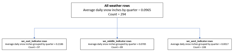
The following decision tree reflects the preceding results regressing each of the three predictors on the snow in inches grouped by quarter. As indicated in the preceding table, the long_dec_degree_one_third_indicator is the name of the predictor that accounts for the greatest variance across rows.
- There are 294 weather rows that are candidates for splitting on the first level of the decision tree regression.
- The category names for the long_dec_degree_one_third_indicator predictor become node names for the first level of the decision tree. These names are:
- we_east_indicator
- we_middle_indicator
- we_west_indicator
- The overall average daily snow is .0965 inches. When the weather rows are split by longitude decimal degrees
- the largest average daily snow is for the weather rows associated with the eastern region
- the smallest average daily snow is for the weather rows associated with the western region
- the middle region has an average daily snow that is in between the largest and smallest amount of snow
- The sample size of 294 weather rows splits across the three first-level nodes:
- 97 rows for the we_east_indicator node
- 89 rows for the we_middle_indicator node
- 108 rows for the we_west_indicator node
Process, code, and results for computing second-level decision tree measures
This section of the tip has four subsections that illustrate key elements of the process and code for adding a second level of nodes to the preceding decision tree. There are two remaining predictors, namely snowy_quarter_indicator and lat_dec_degree_one_third_indicator, for contributing nodes to the second level. You can add either of these candidate predictors to the first-level nodes depending on which predictor has the largest sd_reduction. This section sketches the process and T-SQL code for adding second-level nodes to the decision tree. The section also presents and discusses the decision tree diagram for regression through the second-level nodes.
Setup steps for adding second-level nodes
There are two steps for setting up to add second-level nodes to the first-level nodes of the decision tree.
- First, you create and populate temporary tables based on the rows associated with each of the first-level nodes. Within the context of this tip, this step creates three sets of rows that can be split based on the categories of the two remaining predictors.
- Second, you need to add three sets of local variables for holding and displaying measures that are computed when adding a new set of child nodes to a set of parent nodes. The parent nodes for the second-level nodes are the first-level nodes.
- There is a set of local variables for the parent nodes.
- There are two additional sets of local variables – one set each for each potential set of second-level nodes.
Here is the code creating and populating the three temporary tables based on the first-level nodes. The names of the three temporary tables are: #we_east_indicator_target, #we_middle_indicator_target, and #we_west_indicator_target. The rows in each temporary table is an excerpt from the full set of weather rows.
-- create and populate #we_east_indicator_target
begin try
   drop table #we_east_indicator_target
end try
begin catch
   print '#we_east_indicator_target table not available to drop'
end catch

-- add the regression dataset for #we_east_indicator_target weather records
select *
into #we_east_indicator_target
from #for_sd_reduction_with_date_and_geog_bins
where long_dec_degree_one_third_tile_indicator = 'west_east_east_indicator'
order by STATEPROV, noaa_station_id, [year], [quarter]


-- create and populate #we_middle_indicator_target
begin try
   drop table #we_middle_indicator_target
end try
begin catch
   print '#we_middle_indicator_target table not available to drop'
end catch

-- add the regression dataset for #we_middle_indicator_target weather records
select *
into #we_middle_indicator_target
from #for_sd_reduction_with_date_and_geog_bins
where long_dec_degree_one_third_tile_indicator = 'west_east_middle_indicator'
order by STATEPROV, noaa_station_id, [year], [quarter]


-- create and populate #we_west_indicator_target
begin try
   drop table #we_west_indicator_target
end try
begin catch
   print '#we_west_indicator_target table not available to drop'
end catch

-- add the regression dataset for #we_west_indicator_target weather records
select *
into #we_west_indicator_target
from #for_sd_reduction_with_date_and_geog_bins
where long_dec_degree_one_third_tile_indicator = 'west_east_west_indicator'
order by STATEPROV, noaa_station_id, [year], [quarter]
Here is the declare statement that specifies each of three sets of local variables used to compute the second-level nodes. The three sets are
- The four measures for each of the three first-level nodes have prefixes starting with we_east_indicator, we_middle_indicator, or we_west_indicator
- The four measures for each of the two snowy_quarter category values and the snowy_quarter predictor summary values (@weighted_sd_for_snowy_quarter_indicator and @snowy_quarter_indicator_sd_reduction)
- The four measures for the three north_south predictor categories (ns_north_indicator, ns_middle_indicator, and ns_south_indicator) as well as the corresponding predictor summary values (@weighted_sd_for_lat_dec_degree_one_third_indicator and @lat_dec_degree_one_third_indicator_sd_reduction)
-- declare local variables for sd reduction comps

declare
 @we_east_indicator_mean float, @we_east_indicator_stdevp float, @we_east_indicator_n float, @we_east_indicator_cv float
,@we_middle_indicator_mean float, @we_middle_indicator_stdevp float, @we_middle_indicator_n float, @we_middle_indicator_cv float
,@we_west_indicator_mean float, @we_west_indicator_stdevp float, @we_west_indicator_n float, @we_west_indicator_cv float


,@wintery_q_mean float, @wintery_q_stdevp float, @wintery_q_n float, @wintery_q_cv float
,@non_wintery_q_mean float, @non_wintery_q_stdevp float, @non_wintery_q_n float, @non_wintery_q_cv float
,@weighted_sd_for_snowy_quarter_indicator float, @snowy_quarter_indicator_sd_reduction float

,@ns_north_indicator_mean float, @ns_north_indicator_stdevp float, @ns_north_indicator_n float, @ns_north_indicator_cv float
,@ns_middle_indicator_mean float, @ns_middle_indicator_stdevp float, @ns_middle_indicator_n float, @ns_middle_indicator_cv float
,@ns_south_indicator_mean float, @ns_south_indicator_stdevp float, @ns_south_indicator_n float, @ns_south_indicator_cv float
,@weighted_sd_for_lat_dec_degree_one_third_indicator float, @lat_dec_degree_one_third_indicator_sd_reduction float
Code and results for reporting on the snowy_quarter_indicator
Here is the code for computing the sd reduction for the snowy_quarter_indicator. It computes the sd reduction for the snowy_quarter_indicator in four steps.
- In step 1, it computes and displays the four measures for the root node based on the we_east_indicator. One especially important root node measure populates the @we_east_indicator_stdevp local variable. The computation of the @we_east_indicator_stdevp local variable is based on the rows of the #we_east_indicator_target table.
- In step 2, the code creates and populates a fresh copy of a temporary table named #temp_for_bin_rows; this table is derived from the #we_east_indicator_target table for rows whose snowy_quarter_indicator column value equals wintery quarter. The step next uses the #temp_for_bin_rows table to compute and to display the four measures of the standard deviation reduction process.
- Step 3 truncates the #temp_for_bin_rows table and re-populates it from the #we_east_indicator_target table for rows with snowy_quarter_indicator column values equal to non_wintery quarter. Then, the code uses the #temp_for_bin_rows table to compute and to display the four measures of the standard deviation reduction process.
- Step 4 populates computes and displays the @weighted_sd_for_snowy_quarter_indicator and @snowy_quarter_indicator_sd_reduction local variables.
-- for snowy_quarter_indicator sd reduction

-- step 1: compute, assign, and echo mean, standard, n, and coefficient of determination
-- for target col (snow_avg) based on ns_north_indicator rows

select
 @we_east_indicator_mean = avg(snow_avg)
,@we_east_indicator_stdevp = stdevp(snow_avg)
,@we_east_indicator_n =  count(*)
,@we_east_indicator_cv =(@we_east_indicator_stdevp/@we_east_indicator_mean) * 100
from #we_east_indicator_target

-- echo assignments
select
 @we_east_indicator_mean [@we_east_indicator_mean]
,@we_east_indicator_stdevp [@we_east_indicator_stdevp]
,@we_east_indicator_n [@we_east_indicator_n]
,@we_east_indicator_cv [@we_east_indicator_cv]

-- step 2: compute and assign mean, standard, n, and coefficient of determination
-- for target col (snow_avg) based on wintery quarter rows

-- create and populate #temp_for_bin_rows table
begin try
drop table #temp_for_bin_rows
end try
begin catch
   print 'drop table #temp_for_bin_rows table not available to drop'
end catch


select * into #temp_for_bin_rows
from #we_east_indicator_target
where snowy_quarter_indicator = 'wintery quarter'

select
 @wintery_q_mean = avg(snow_avg)
,@wintery_q_stdevp = stdevp(snow_avg)
,@wintery_q_n =  count(*)
,@wintery_q_cv =(@wintery_q_stdevp/@wintery_q_mean) * 100

from #temp_for_bin_rows

-- echo assignments
select
 @wintery_q_mean [@wintery_q_mean]
,@wintery_q_stdevp [@wintery_q_stdevp]
,@wintery_q_n [@wintery_q_n]
,@wintery_q_cv [@wintery_q_cv]

-- step 3: compute and assign mean, standard, n, and coefficient of determination
-- for target col (snow_avg) based on non_wintery quarter rows

-- clear #temp_for_bin_rows table
truncate table #temp_for_bin_rows

-- freshly populate #temp_for_bin_rows table with non_wintery rows
insert into #temp_for_bin_rows
select *  from #we_east_indicator_target where snowy_quarter_indicator = 'non_wintery quarter'
--select * from #temp_for_bin_rows

-- compute and assign mean, standard, n, and coefficient of determination
-- for target col (snow_avg) for non_wintery population
select
 @non_wintery_q_mean = avg(snow_avg)
,@non_wintery_q_stdevp = stdevp(snow_avg)
,@non_wintery_q_n =  count(*)
,@non_wintery_q_cv =(@non_wintery_q_stdevp/@non_wintery_q_mean) * 100
from #temp_for_bin_rows

-- echo assignments
select
 @non_wintery_q_mean [@non_wintery_q_mean]
,@non_wintery_q_stdevp [@non_wintery_q_stdevp]
,@non_wintery_q_n [@non_wintery_q_n]
,@non_wintery_q_cv [@non_wintery_q_cv]

-- step 4: compute and display @weighted_sd_for_snowy_quarter_indicator
-- and @snowy_quarter_indicator_sd_reduction

set @weighted_sd_for_snowy_quarter_indicator =
(@wintery_q_n/@we_east_indicator_n)*@wintery_q_stdevp
+
(@non_wintery_q_n/@we_east_indicator_n)*@non_wintery_q_stdevp

set @snowy_quarter_indicator_sd_reduction =
@we_east_indicator_stdevp - @weighted_sd_for_snowy_quarter_indicator

select
 @weighted_sd_for_snowy_quarter_indicator [@weighted_sd_for_snowy_quarter_indicator]
,@snowy_quarter_indicator_sd_reduction [@snowy_quarter_indicator_sd_reduction]
The following screen shot shows the four results sets from the preceding script.
- The first results set is for the root node, which in this case has 97 weather rows in the #we_east_indicator_target table. The mean amount of snow over the 97 rows is 0.218663592476239 inches.
- The second results set is for the processing of #we_east_indicator_target table rows with snowy_quarter_indicator value of wintery_quarter. There are 47 rows meeting this criterion. The rows meeting this criterion have a mean amount of snow equal to 0.424088339451973 inches. This is the predicted value for these 47 rows.
- The predicted mean amount of snow is 0.0255643303190481 inches for the 50 rows having a snowy_quarter_indicator value of non_wintery_quarter.

The following screen shot shows comparable results sets for making predictions with the @lat_dec_degree_one_third_indicator predictor category values (i.e., ns_north_indicator, ns_middle_indicator, and ns_south_indicator). Notice there is no row for the set of all rows from the #we_east_indicator_target table. The results sets below draw on the same table as in the preceding screen shot.
The most important point to observe for the following results sets is that the standard deviation reduction value in the last row has a value of NULL. This means the sd reduction value is missing. Therefore, the @lat_dec_degree_one_third_indicator predictor is disqualified for making predictions for rows in the #we_east_indicator_target table.
The reason the @lat_dec_degree_one_third_indicator standard deviation reduction is NULL is because there are no rows for the third category (@ns_south_indicator_n = 0) of the lat_dec_degree_one_third_indicator predictor. As a result, the mean for the third category is NULL. Furthermore, NULL values propagate in T-SQL code so the NULL value for @ns_south_indicator_mean propagates to the @weighted_sd_for_lat_dec_degree_one_third_indicator and @lat_dec_degree_one_third_indicator_sd_reduction local variables.

Diagram through the second level for the decision tree regression model
The T-SQL script in the download for this tip extends the approach for all second-level nodes in the decision tree regression model. The diagram for all second-level nodes appears in the screen shot below.
- Each of the three first-level nodes is split into two nodes based on the two category values for the snowy_quarter_indicator.
- The decision tree never shows a split of a first-level node based on the lat_dec_degree_one_third_indicator category values. This is because the sd reduction value for lat_dec_degree_one_third_indicator predictor is NULL for all second-level nodes.
- The NULL values for standard deviation reduction values are not the result of errors. Instead, they reflect the distribution of data values across lat_dec_degree_one_third_indicator category values. If you encounter this situation with your data, you can remedy it by adjusting category boundaries so that all categories have some observations in them.
- Notice that the sum of the rows associated with second-level nodes always equals the number of rows in their first-level parent node. This is a check for the validity of the outcome.
- Also, the mean snow amount for a first-level parent node always falls in between the mean snow amount for its second-level child nodes.

Next Steps
This tip is for anyone with a basic understanding of T-SQL and an interest in learning about the decision tree algorithm for regressing multiple predictor columns on a target column. After walking through the steps in this tip, you can see the decision tree regression algorithm is not especially complicated. The hardest part of the algorithm presented in this tip may be the devising of a naming convention for keeping track of parent and child tables as well as scalar values required by the algorithm.
There are three files in the download for this tip.
- Running the sql file from end-to-end generates the results sets reported in this tip if you have the SQL Server weather warehouse referenced in this tip. This previous tip describes how to create and populate the weather warehouse.
- There is one Excel workbook file that contains three tabs with data for selected temporary tables referenced in this tip.
- One tab contains the data in the #source_data table. The data shows output from the first script in the “Data for this tip” section.
- A second tab contains the data in the #temp table. The data in this tab shows a table with multiple predictor columns and a partition column to facilitate percentile computations across all rows for predictor columns.
- A third tab contains data for the #for_sd_reduction_with_date_and_geog_bins table. This table is the base table for submittal to the decision tree regression algorithm example walked through in this tip.
- One PowerPoint file with two slides containing the two decision trees presented in the tip.
The decision tree regression algorithm is a very commonly used data science algorithm for predicting the values in a target column of a table from two or more predictor columns in a table. Here are two additional references for you to review for learning more about the algorithm.
After you apply the technique to the sample data for this tip, you will be ready to apply the decision tree regression algorithm to data from your organization. If you have ever been stumped about how to predict a target column of values from two or more predictor columns, you will know how to do it after reviewing the content in this tip. Furthermore, if you are working with a team of data scientists, the information that you gain from this tip will enable you to add more value to data science projects and expose you to general kinds of issues that you are likely to encounter with data science models.

Rick Dobson is a SQL Server professional with decades of T-SQL experience that includes authoring books, running a national seminar practice, working for businesses on finance and healthcare development projects, and serving as a regular contributor to MSSQLTips.com. He has been a practicing Python developer for more than the past half decade – with a special emphasis for data visualization and ETL tasks with JSON and CSV files. His most recent professional passions include financial time series data and analyses, AI models, and statistics. If you are interested in growing your skills in any of these areas especially as they relate to financial securities, consider visiting his blog at https://securitytradinganalytics.blogspot.com/2023/12/.
- MSSQLTips Awards: Leadership (200+ tips) – 2025 | Author of the Year Contender – 2017-2024


