Problem
I want to grow my understanding of decision tree models for classifying objects. Please present T-SQL code and a framework that can classify objects from a dataset and assign the objects to nodes in a decision tree. Please also contrast the use of T-SQL code for binomial as well as multinomial classification.
Solution
Decision trees are a data science technique for identifying criteria based on a set of attributes that classify objects as belonging to one of two or more groups. Objects to classify can include prospective heart-disease patients. The decision tree can assess if a patient has heart disease or not. Another use case for a decision tree model is to assess if a prospective borrower qualifies for an especially low-interest-rate loan, a higher-interest-rate loan, or no loan at all.
This tip and the series to which it belongs illustrates the basics of how to implement classic data science models with T-SQL. The purpose of the tip series is to introduce T-SQL developers to selected data science models. To facilitate this goal, models are built with T-SQL code.
The decision tree algorithm for classifying objects
This tip builds on a prior tip titled T-SQL Code for the Decision Tree Algorithm – Part 1. Among the enhancements in this tip are the building of a multi-level decision tree instead of one with just a root node followed by two nodes right below the root node. If you would like an introduction to core decision tree model architecture, refer to the part 1 tip in this series on decision trees. Another enhancement of this tip is an introduction to concepts for building multinomial decision tree sets.
A decision tree model starts with all dataset objects belonging to a root node.
- Then, the decision tree algorithm discovers a criterion based on an attribute that is best at splitting the dataset into two nodes directly below the root node. The algorithm includes rules for finding a criterion that segments the root node dataset rows into two groups of rows that are as homogeneous as possible.
- Each attribute in the dataset can have a weighted gini score.
- The weighted gini score assesses the purity of the nodes resulting from a splitting criterion based on an attribute. The lower the weighted gini score, the purer the resulting nodes after a split.
- The attribute with the lowest gini score can be used to specify a criterion that splits the root node objects so that the resulting nodes are purer than any other pair of nodes below the root.
- Next, each of the two nodes below the root node is a candidate for being split into two other nodes.
- If one of the nodes below the root node contains objects of just one type, then there is no need to split it because it is already perfectly pure.
- Presuming both nodes below the root node can be split, each of the four nodes at the second level below the root node can be either parent or leaf nodes.
- A leaf node is one that has no nodes below it. For example, a leaf node could have only one type of object associated with it.
- A parent node can be split into two additional nodes by a new criterion.
- If the weighted gini score for the purity of a pair of child nodes is greater than their parent node (that is, less pure), then those child nodes can be disregarded. In this case, the parent node converts to a leaf node.
- If the weighted gini score for the child nodes is less than for its parent node, then each of the newly split nodes can be split again like its parent.
- You can successively split the nodes on any level until all nodes on a level are leaf nodes or until there are no more attributes available for splitting.
- Depending on the relationships of attributes and objects in the dataset you are processing, you may want to cease splitting nodes or remove previously split nodes. This final step can sometimes improve the ability of a decision tree classification model successfully classifying objects from more datasets.
This tip demonstrates the use of the weighted gini score to assess the purity of the two nodes below a root node or a parent node. There are other metrics for assessing the purity of the rows assigned to a pair of nodes, but the weighted gini score is especially easy to program and fast to compute.
A classic decision tree has just two types of objects in a dataset – a patient is a good candidate for treatment with a procedure, such as an operation, or a patient is not a good candidate for that type of operation.
- This kind of classic decision tree assigns each object to one of two objects. This is an example of binomial classification.
- However, sometimes you may encounter situations where you need to assign objects to more than two classes. This is called multinomial classification.
Multinomial classification can be treated as an extension of binomial classification with a one-versus-rest approach. For example, if you need to assign objects to one of three groups (class A, class B, or class C), you can use three decision tree models. Each of the three decision tree models performs a different binomial classification.
- In the first decision tree, the binomial choice can be for an object belonging to class A or either classes B or C.
- In the second decision tree, the binomial choice can be for an object belonging to class B or either classes A or C.
- In the third decision tree, the binomial choice can be for an object belonging to class C or either classes A or B.
After you classify each object with each of the three decision tree models, you can compute the probability of each object being classified to each class across all three decision tree models. There are multiple data science techniques for processing the output from three or more decision tree models to find the class for which each object most likely belongs. These techniques (see here and here for detail about these techniques) are beyond the scope of this tip. However, this tip does demonstrate techniques for specifying and populating multiple decision trees for multinomial classification.
The data for this tip
This tip builds decision tree models for analytically classifying weather observations by state from a SQL Server weather warehouse. The source for the observations is the National Oceanic and Atmospheric Administration (NOAA) website. The weather facts are minimum daily temperature in Fahrenheit degrees, inches of daily rain, and inches of daily snow. The weather observations come from a previous tip that creates and populates a SQL Server weather warehouse.
It is common for data science projects to begin with a data wrangling process. The project in this tip starts the wrangling by pulling an excerpt from a weather data warehouse. To keep the tip’s focus on classification models, T-SQL code for data wrangling is summarized at an overview level in this tip. The detailed code along with intermediate output tables are available in this tip’s download. The code starts by extracting data for a dataset with class identifiers and weather facts as attributes. The warehouse includes daily weather over a four-year period (2016 – 2019) for weather stations from five states (California, Florida, Illinois, New York, and Texas). Key tables from the database include a couple of fact tables with references to two dim tables.
- The fact tables are named FactWeather and FactStation.
- Weather observations are made at weather stations. A weather station is identified by a station identifier (noaa_station_id) and state jurisdiction (STATEPROV) in which a station resides. The FactStation table includes these two facts along with others for weather stations.
- The FactWeather table stores weather facts, such as tmin (minimum daily temperature in Fahrenheit degrees), prcp (daily rain in inches), and snow (snow in inches).
- For simplicity, the code links the noaa_station_id column values from the FactWeather table to the noaa_station_id column values from the FactStation table. The warehouse has a DimStation table, which serves as a master list of station identifier values along with station names.
- The year and quarter in which weather observations were made are extracted from the DimDate table. The date foreign key in the FactWeather table points at the date primary key in the DimDate table.
- The average daily weather observations were grouped by state, station identifier, year, and quarter.
- The counts in the following results set image reflect the number of averaged weather observations by state. The three states with the largest number of averaged quarterly observations are Texas, New York, and Illinois. There are 227 (91 + 78 + 58) averaged quarterly observations for these three states. This tip’s analysis of the weather data is restricted to these 227 rows of averaged quarterly weather observations per state.

The table below shows images of the first and last five weather data rows from each state. For the images below, the grouped average daily weather observation numerical values were further transformed based on whether weather facts were at or below the median value for an attribute or above the median value for an attribute. These transformed data are from a table named for_gini_comps_with_median_based_bins. A casual review of the rows from the three states in the table facilitate a confirmation of the row counts by state. In addition, the review supports potential weather pattern differences between the states.
- The fifty-eight rows from IL have row numbers 1 through 58. The seventy-eight rows from NY have row numbers of 59 through 136. Finally, there are ninety-one rows from TX with row numbers of 137 through 227.
- It is snowier and colder in NY than the other two states because nine of the ten rows from NY have quarterly average snow weather observations that are above the median for all three states. Also, NY is likely to have quarterly average minimum daily temperatures below the median minimum daily temperature of all three states.
- In contrast, the weather rows point to warmer weather in TX because TX generally has quarterly median minimum daily temperatures that are above the median minimum daily temperature of all three states.
| Rows Label | Selected rows from three states |
|---|---|
| First 5 from IL |  |
| Last 5 from IL |  |
| First 5 from NY |  |
| Last 5 from NY |  |
| First 5 from TX | 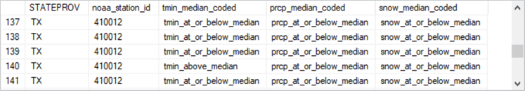 |
| Last 5 from TX |  |
In-depth look at first-level split for NY vs. IL & TX decision tree
This section offers a walk-through of the steps for deriving the first-level nodes below a root node in a decision tree from the data source described in the preceding section. The decision tree is based on a one-versus-rest classification model formulation.
- The one is for NY.
- The rest is for IL & TX.
Weighted gini scores for the first-level split
To split the root node, you need to find the lowest weighted gini score from among the three attributes available for splitting the root node. In the preceding table, you can see the three attributes have names of tmin_median_coded, prcp_median_coded, and snow_median_coded values. Each of these attributes have just two value types – above the median and at or below the median. The weighted gini score that is lowest across all three attributes is best at distinguishing NY rows from the rows for both IL & TX.
Here are the computed weighted gini scores for distinguishing two nodes directly below the root node. As you can see, the snow_median_coded attribute is best at distinguishing the rows associated with NY from the rows associated with IL & TX.
| Attribute name | Weighted gini score |
|---|---|
| tmin_median_coded | 0.4281 |
| prcp_median_coded | 0.4469 |
| snow_median_coded | 0.3703 |
Eight steps for computing weighted gini score for snow median coded values
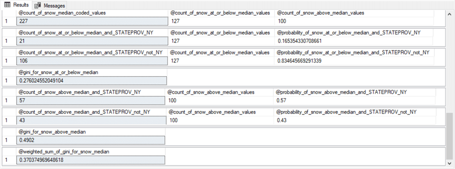
The screen shot below shows eight steps for computing the weighted gini score (@gini_for_snow_at_or_below_median) for snow_median_coded attribute values. Each step is a separate results set from code like that presented and discussed in the next sub-section. The eight results sets appear at the end of this sub-section.
- The first results set splits the 227 rows associated with the root node (@count_of_snow_median_coded_values) into two nodes: the 127 rows at or below the median value (@count_of_snow_at_or_below_median_values) and the 100 rows above the median value (@count_of_snow_above_median_values).
- The second and third results sets compute two probabilities.
- 21 rows of the 127 rows at or below the median snow value are from NY. This means that there is just a 16.5 percent chance (21/127) of a NY row being at or below the snow median (@probability_of_snow_at_or_below_median_and_STATEPROV_NY).
- On the other hand, there are 106 rows at or below the median snow value that are from either IL or TX. This means there is an 83.5 percent chance (106/127) of a row from the IL & TX class being at or below the median snow value (@probability_of_snow_at_or_below_median_and_STATEPROV_not_NY).
- The fourth step is to compute the gini score for being at or below the snow median (@gini_for_snow_at_or_below_median). The expression for the gini score is:
1 – (@probability_of_snow_at_or_below_median_and_STATEPROV_NY2 + @probability_of_snow_at_or_below_median_and_STATEPROV_not_NY2)
- The fifth and sixth results sets compute two other probabilities.
- 57 rows of the 100 rows above the median snow value are from NY. This means that 57 percent of the rows above the median are from NY (@probability_of_snow_above_median_and_STATEPROV_NY).
- The remaining 43 rows with snow values above the median are from the IL & TX class. This means that 43 percent of the rows with snow values above the median are from the IL & TX class (@probability_of_snow_above_median_and_STATEPROV_not_NY).
- The seventh step is to compute the gini score for being above the snow median (@gini_for_snow_above_median). The expression for the gini score is:
1 – (@probability_of_snow_above_median_and_STATEPROV_NY2 + @probability_of_snow_above_median_and_STATEPROV_not_NY2)
- The eighth step computes the weighted gini score for snow median coded values as a weighted average of the @gini_for_snow_at_or_below_median value and the @gini_for_snow_above_median value. The weights are based on the relative proportion of rows at or below the median snow value versus the proportion of rows above the median snow value. The expression in terms of the values from earlier steps is:
((@count_of_snow_at_or_below_median_values/@count_of_snow_median_coded_values) * @gini_for_snow_at_or_below_median)
+
((@count_of_snow_above_median_values/@count_of_snow_median_coded_values) * @gini_for_snow_above_median)
T-SQL code for eight steps
The following T-SQL script can generate the results sets described in the preceding sub-section for snow median coded values. There are three main segments to the script.
- The first segment configures the environment to perform the sequence of steps that end in the computation of the weighted gini score for snow median coded values.
- The script starts with a use statement for the DataScience database. The script logic does not depend rigidly on that database name; use whatever name suits your circumstances.
- However, the script does require the for_gini_comps_with_median_based_bins table in whatever database you decide to test the script. Excerpts from this table are displayed and discussed in section named “The data for this tip”.
- The first select statement in the first segment creates and populates the for_gini_comps_snow_median table from the for_gini_comps_with_median_based_bins table. The select statement code designates three columns for the for_gini_comps_snow_median table: STATEPROV, noaa_station_id, and snow_median_coded.
- The second script section is separated from the first section by a line of comment markers.
- This section includes a series of declare statements for local variables.
- The values for these local variables are populated by select statements and expressions.
- The first local variable, @count_of_snow_median_coded_values, returns the count of median coded snow values – namely, 227.
- The last local variable, @weighted_sum_of_gini_for_snow_median, computes the weighted gini score for median coded snow values. This local variable value is presented, along with two other weighted gini score values, in the sub-section named “Weighted gini scores for the first-level split”. The T-SQL code for the other two weighted gini score values is available in the download for this tip.
- The third script section is separated from the second section by a line of comment markers. This section consists of a series of select statements to display the local variable values populated in the second section.
use DataScience
go

-- Decision Tree Model for NY vs. TX & IL
-- from root node


begin try
   drop table dbo.for_gini_comps_snow_median
end try
begin catch
   print 'for_gini_comps_snow_median table not available to drop'
end catch


-- insert into snow_median_coded with STATEPROV and noaa_station_id identifiers
select STATEPROV, noaa_station_id, snow_median_coded
into dbo.for_gini_comps_snow_median
from dbo.for_gini_comps_with_median_based_bins
order by STATEPROV, noaa_station_id

---------------------------------------------------------------------------------------------------------------

declare
 @count_of_snow_median_coded_values float =
(select count(snow_median_coded) [count_of_snow_median_coded values]
from dbo.for_gini_comps_snow_median)

,@count_of_snow_at_or_below_median_values float =
(select count(snow_median_coded) [count_of_tmin_at_or_below_median values]
from dbo.for_gini_comps_snow_median
where snow_median_coded = 'snow_at_or_below_median')

,@count_of_snow_above_median_values float =
(select count(snow_median_coded) [count_of_snow_above_median values]
from dbo.for_gini_comps_snow_median
where snow_median_coded = 'snow_above_median')

,@count_of_snow_at_or_below_median_and_STATEPROV_NY float =
(select count(*) [count of snow_median_coded = 'snow_at_or_below_median' and STATEPROV = 'NY']
from dbo.for_gini_comps_snow_median
where snow_median_coded = 'snow_at_or_below_median' and STATEPROV = 'NY')

,@count_of_snow_at_or_below_median_and_STATEPROV_not_NY float =
 (select count(*) [count of snow_median_coded = 'snow_at_or_below_median' and STATEPROV != 'NY']
from dbo.for_gini_comps_snow_median
where snow_median_coded = 'snow_at_or_below_median' and STATEPROV != 'NY')


declare
 @probability_of_snow_at_or_below_median_and_STATEPROV_NY float =
 (select @count_of_snow_at_or_below_median_and_STATEPROV_NY
  /
  @count_of_snow_at_or_below_median_values)
,@probability_of_snow_at_or_below_median_and_STATEPROV_not_NY float =
 (select @count_of_snow_at_or_below_median_and_STATEPROV_not_NY
  /
  @count_of_snow_at_or_below_median_values )


declare
 @gini_for_snow_at_or_below_median float =
  1 -(power(@probability_of_snow_at_or_below_median_and_STATEPROV_NY,2) + power(@probability_of_snow_at_or_below_median_and_STATEPROV_not_NY,2))

declare
@count_of_snow_above_median_and_STATEPROV_NY float =
(select count(*) [count of snow_median_coded = 'snow_above_median' and STATEPROV = 'NY']
from dbo.for_gini_comps_snow_median
where snow_median_coded = 'snow_above_median' and STATEPROV = 'NY')

,@count_of_snow_above_median_and_STATEPROV_not_NY float =
 (select count(*) [count of snow_median_coded = 'snow_above_median' and STATEPROV != 'NY']
from dbo.for_gini_comps_snow_median
where snow_median_coded = 'snow_above_median' and STATEPROV != 'NY')


declare
 @probability_of_snow_above_median_and_STATEPROV_NY float =
 (select @count_of_snow_above_median_and_STATEPROV_NY
  /
  @count_of_snow_above_median_values)
,@probability_of_snow_above_median_and_STATEPROV_not_NY float =
 (select @count_of_snow_above_median_and_STATEPROV_not_NY
  /
  @count_of_snow_above_median_values )


declare
 @gini_for_snow_above_median float =
  1 -(power(@probability_of_snow_above_median_and_STATEPROV_NY,2) + power(@probability_of_snow_above_median_and_STATEPROV_not_NY,2))

declare
 @weighted_sum_of_gini_for_snow_median float =
 ((@count_of_snow_at_or_below_median_values/@count_of_snow_median_coded_values) * @gini_for_snow_at_or_below_median)
  +
 ((@count_of_snow_above_median_values/@count_of_snow_median_coded_values) * @gini_for_snow_above_median)

select
 @count_of_snow_median_coded_values [@count_of_snow_median_coded_values]
,@count_of_snow_at_or_below_median_values [@count_of_snow_at_or_below_median_values]
,@count_of_snow_above_median_values [@count_of_snow_above_median_values]

select
 @count_of_snow_at_or_below_median_and_STATEPROV_NY [@count_of_snow_at_or_below_median_and_STATEPROV_NY]
,@count_of_snow_at_or_below_median_values [@count_of_snow_at_or_below_median_values]
,@probability_of_snow_at_or_below_median_and_STATEPROV_NY [@probability_of_snow_at_or_below_median_and_STATEPROV_NY]

select
 @count_of_snow_at_or_below_median_and_STATEPROV_not_NY [@count_of_snow_at_or_below_median_and_STATEPROV_not_NY]
,@count_of_snow_at_or_below_median_values [@count_of_snow_at_or_below_median_values]
,@probability_of_snow_at_or_below_median_and_STATEPROV_not_NY [@probability_of_snow_at_or_below_median_and_STATEPROV_not_NY]

select @gini_for_snow_at_or_below_median [@gini_for_snow_at_or_below_median]

select
 @count_of_snow_above_median_and_STATEPROV_NY [@count_of_snow_above_median_and_STATEPROV_NY]
,@count_of_snow_above_median_values [@count_of_snow_above_median_values]
,@probability_of_snow_above_median_and_STATEPROV_NY [@probability_of_snow_above_median_and_STATEPROV_NY]

select
 @count_of_snow_above_median_and_STATEPROV_not_NY [@count_of_snow_above_median_and_STATEPROV_not_NY]
,@count_of_snow_above_median_values [@count_of_snow_above_median_values]
,@probability_of_snow_above_median_and_STATEPROV_not_NY [@probability_of_snow_above_median_and_STATEPROV_not_NY]

select @gini_for_snow_above_median [@gini_for_snow_above_median]

---------------------------------------------------------------------------------------------------------------

select @weighted_sum_of_gini_for_snow_median [@weighted_sum_of_gini_for_snow_median]
The decision tree for the first-level split
The following diagram shows the decision tree for the NY rows versus the IL & TX rows from the root node and after the first split.
- The root node has 78 NY rows and 149 rows from both IL & TX. Therefore, about two-third of the root node rows are from IL & TX rows, and about one-third of the root node rows are classified as NY rows.
- There are two nodes at the first-level split below the root node. The split is on the snow criterion.
- The node on the left is for rows with a snow median coded value at or below the median snow value.
- The node on the right is for rows with a snow median coded value above the median snow value.
- The node with rows at or below the median snow value (on the left) has just 21 rows from NY and 106 rows from IL & TX. About 16 percent of its rows are from NY. In contrast, the same node has about 84 percent of its rows from IL & TX.
- The node with rows above the median snow value (on the right) has 57 rows from NY and just 43 rows from IL & TX. Nearly 60 percent of the rows for this node are from NY, and slightly more than 40 percent of this node’s rows are from IL & TX.
- Clearly, the first-level split after the root node was highly effective at splitting the root node’s rows into two row sets that were more homogeneous by one and rest classification names than the rows associated in the root node. However, the first-level nodes are not perfectly pure, and there are two remaining candidate attributes in the source dataset on which to perform a second-level split.

Look at second-level split for NY vs. IL and TX decision tree
The sub-sections in this section adapt the approach for splitting the root node rows into two first-level nodes so that each first-level node can be split into up to two second-level nodes.
- The first sub-section starts with a focus on the weighted gini scores for picking the best attribute for splitting first-level nodes into second-level nodes.
- The second sub-section presents T-SQL code for splitting the first-level nodes, and this section displays selected results sets for splitting first-level nodes into second-level nodes.
- The third sub-section maps values from selected results sets displayed in the second sub-section to an updated version of the preceding decision tree diagram that shows nodes for the first two levels below the root node.
Weighted gini scores for the second-level split
The second-level split builds on the first-level split.
- That is, each of the nodes from the first level split are candidates for splitting into two more nodes.
- However, sometimes a first-level node should not be split.
- This can happen because a first-level node has just one type object associated with it.
- Also, a first-level node should not be split when the weighted gin scores for candidate second-level nodes are greater than the weighted gini score for the first-level split of the root node.
The following screen shot shows second-level weighted gini scores in column D along with other relevant reference data in the remaining columns. Remember, the lower the weighted gini score, the purer the rows associated with a node.
- A second-level pair of nodes can be derived for each first-level node. Each member of a second-level pair of nodes has a different attribute than the attribute for the first-level split. In this tip example, candidate attributes for a second-level split are tmin median coded values or prcp median coded values.
- The weighted gini score for the first level split (column C) is the same for all rows because the following table has rows for just the best candidate attribute (snow) for splitting rows at the first level. The weighted gini score for the first-level split is .3703.
- The best candidate attribute for splitting at the second level can be either tmin or prcp. By convention in this tip, splits are made relative to the overall median value for a candidate attribute with designations of at or below the median or above the median. You can optionally designate other bin categories if you prefer.
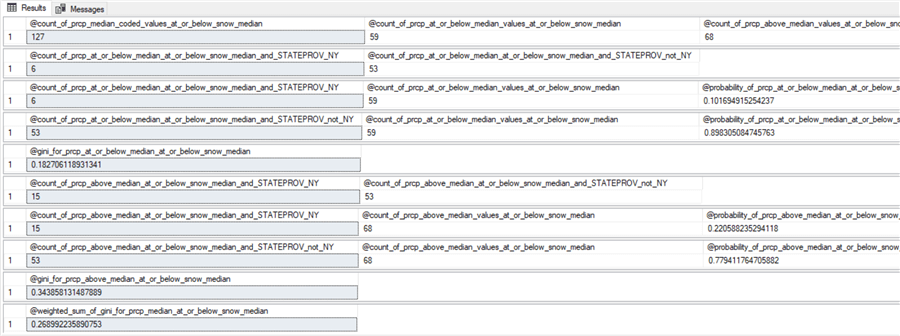
- The best attribute for splitting the rows whose snow values are at or below the median snow value is the prcp attribute. Its weighted gini score is .2689, which is slightly less than .2705 for the tmin attribute. The weighted gini score of .2689 is also the best splitting attribute of the first first-level split node because its value is lower than the weighted gini score for the first-level node at or below the median snow value.
- The second node at the first level is for rows above the median snow value. The weighted gini scores for a split of this second first-level node are larger than for the weighted gini score for the first-level split. Therefore, there is no value gained by splitting the second first-level node.

T-SQL code and results sets for eight steps
The following script shows the T-SQL code for computing the weighted gini score for splitting based on the prcp attribute in the second level below the at or below snow median node from the first-level split. There are two key points that you may find especially useful to study.
- The code for creating and populating the for_gini_comps_at_or_below_snow_median_for_prcp table has the columns for computing the weighted gini score for splitting the first node from the first-level split. The snow_median_coded column is for filtering the desired set of rows for splitting. The prcp_median_coded column is for performing the split based on the best candidate attribute for splitting – namely, prcp. Of course, the for_gini_comps_at_or_below_snow_median_for_prcp table also has a prcp_median_coded values column, which is the column for splitting the first-level node into two second-level nodes.
- Also, the select statement for populating the for_gini_comps_at_or_below_snow_median_for_prcp table has a different design than for the first-level split. In particular, the select statement includes a where clause that filters for rows from the for_gini_comps_with_median_based_bins table that are at or below the median snow value from the first-level split.
- The remainder of the script declares and populates local variables for the eight results sets that conclude with the computation of the weighted gini score for splitting the beginning first-level node with the prcp attribute into two second-level nodes.
- The difference of this code compared to the code for the best first-level split is that declare statements for local variables are immediately followed by select statements for creating one of the eight results sets. The comparable code for the first-level split declares local variables for all results sets before specifying select statements for any of the results sets.
- I did not notice a significant difference in performance time between either approach.
-- Decision Tree Model for NY vs. TX & IL
-- for prcp from at or below snow median parent

begin try
   drop table for_gini_comps_at_or_below_snow_median_for_prcp
end try
begin catch
   print 'for_gini_comps_at_or_below_snow_median_for_prcp table not available to drop'
end catch

-- for dbo.for_gini_comps_from_at_or_below_snow_parent
select STATEPROV, noaa_station_id, snow_median_coded, prcp_median_coded
into for_gini_comps_at_or_below_snow_median_for_prcp
from dbo.for_gini_comps_with_median_based_bins
where snow_median_coded = 'snow_at_or_below_median'
order by STATEPROV, noaa_station_id

-- code for section 1 results set
declare
 @count_of_prcp_median_coded_values_at_or_below_snow_median float =
(select count(prcp_median_coded) [count_of_prcp_median_coded values]
from dbo.for_gini_comps_at_or_below_snow_median_for_prcp)

,@count_of_prcp_at_or_below_median_values_at_or_below_snow_median float =
(select count(prcp_median_coded) [count_of_prcp_at_or_below_median values]
from dbo.for_gini_comps_at_or_below_snow_median_for_prcp
where prcp_median_coded = 'prcp_at_or_below_median')

,@count_of_prcp_above_median_values_at_or_below_snow_median float =
(select count(prcp_median_coded) [count_of_prcp_above_median values]
from dbo.for_gini_comps_at_or_below_snow_median_for_prcp
where prcp_median_coded = 'prcp_above_median')

select
 @count_of_prcp_median_coded_values_at_or_below_snow_median [@count_of_prcp_median_coded_values_at_or_below_snow_median]
,@count_of_prcp_at_or_below_median_values_at_or_below_snow_median [@count_of_prcp_at_or_below_median_values_at_or_below_snow_median]
,@count_of_prcp_above_median_values_at_or_below_snow_median [@count_of_prcp_above_median_values_at_or_below_snow_median]

---------------------------------------------------------------------------------------------------

-- code for section 2 and 3 results sets
declare
@count_of_prcp_at_or_below_median_at_or_below_snow_median_and_STATEPROV_NY float =
(select count(*) [count of prcp_median_coded = 'prcp_at_or_below_median' and STATEPROV = 'NY']
from dbo.for_gini_comps_at_or_below_snow_median_for_prcp
where prcp_median_coded = 'prcp_at_or_below_median' and STATEPROV = 'NY')

,@count_of_prcp_at_or_below_median_at_or_below_snow_median_and_STATEPROV_not_NY float =
(select count(*) [count of prcp_median_coded = 'prcp_at_or_below_median' and STATEPROV != 'NY']
from dbo.for_gini_comps_at_or_below_snow_median_for_prcp
where prcp_median_coded = 'prcp_at_or_below_median' and STATEPROV != 'NY')

select
 @count_of_prcp_at_or_below_median_at_or_below_snow_median_and_STATEPROV_NY [@count_of_prcp_at_or_below_median_at_or_below_snow_median_and_STATEPROV_NY]
,@count_of_prcp_at_or_below_median_at_or_below_snow_median_and_STATEPROV_not_NY [@count_of_prcp_at_or_below_median_at_or_below_snow_median_and_STATEPROV_not_NY]


declare
 @probability_of_prcp_at_or_below_median_at_or_below_snow_median_and_STATEPROV_NY float =
 (select @count_of_prcp_at_or_below_median_at_or_below_snow_median_and_STATEPROV_NY
  /
  @count_of_prcp_at_or_below_median_values_at_or_below_snow_median)
,@probability_of_prcp_at_or_below_median_at_or_below_snow_median_and_STATEPROV_not_NY float =
 (select @count_of_prcp_at_or_below_median_at_or_below_snow_median_and_STATEPROV_not_NY
  /
  @count_of_prcp_at_or_below_median_values_at_or_below_snow_median)

select
 @count_of_prcp_at_or_below_median_at_or_below_snow_median_and_STATEPROV_NY [@count_of_prcp_at_or_below_median_at_or_below_snow_median_and_STATEPROV_NY]
,@count_of_prcp_at_or_below_median_values_at_or_below_snow_median [@count_of_prcp_at_or_below_median_values_at_or_below_snow_median]
,@probability_of_prcp_at_or_below_median_at_or_below_snow_median_and_STATEPROV_NY [@probability_of_prcp_at_or_below_median_at_or_below_snow_median_and_STATEPROV_NY]

select
 @count_of_prcp_at_or_below_median_at_or_below_snow_median_and_STATEPROV_not_NY [@count_of_prcp_at_or_below_median_at_or_below_snow_median_and_STATEPROV_not_NY]
,@count_of_prcp_at_or_below_median_values_at_or_below_snow_median [@count_of_prcp_at_or_below_median_values_at_or_below_snow_median]
,@probability_of_prcp_at_or_below_median_at_or_below_snow_median_and_STATEPROV_not_NY [@probability_of_prcp_at_or_below_median_at_or_below_snow_median_and_STATEPROV_not_NY]

---------------------------------------------------------------------------------------------------

-- code for section 4 results set
declare
 @gini_for_prcp_at_or_below_median_at_or_below_snow_median float =
  1 -(power(@probability_of_prcp_at_or_below_median_at_or_below_snow_median_and_STATEPROV_NY,2)
   + power(@probability_of_prcp_at_or_below_median_at_or_below_snow_median_and_STATEPROV_not_NY,2))


select @gini_for_prcp_at_or_below_median_at_or_below_snow_median [@gini_for_prcp_at_or_below_median_at_or_below_snow_median]

---------------------------------------------------------------------------------------------------

-- code for section 5 and 6 results sets
declare
@count_of_prcp_above_median_at_or_below_snow_median_and_STATEPROV_NY float =
(select count(*) [count of prcp_median_coded = 'prcp_at_or_below_median' and STATEPROV = 'NY']
from dbo.for_gini_comps_at_or_below_snow_median_for_prcp
where prcp_median_coded = 'prcp_above_median' and STATEPROV = 'NY')

,@count_of_prcp_above_median_at_or_below_snow_median_and_STATEPROV_not_NY float =
(select count(*) [count of prcp_median_coded = 'prcp_at_or_below_median' and STATEPROV != 'NY']
from dbo.for_gini_comps_at_or_below_snow_median_for_prcp
where prcp_median_coded = 'prcp_above_median' and STATEPROV != 'NY')

select
 @count_of_prcp_above_median_at_or_below_snow_median_and_STATEPROV_NY [@count_of_prcp_above_median_at_or_below_snow_median_and_STATEPROV_NY]
,@count_of_prcp_above_median_at_or_below_snow_median_and_STATEPROV_not_NY [@count_of_prcp_above_median_at_or_below_snow_median_and_STATEPROV_not_NY]


declare
 @probability_of_prcp_above_median_at_or_below_snow_median_and_STATEPROV_NY float =
 (@count_of_prcp_above_median_at_or_below_snow_median_and_STATEPROV_NY
  /
  @count_of_prcp_above_median_values_at_or_below_snow_median)
,@probability_of_prcp_above_median_at_or_below_snow_median_and_STATEPROV_not_NY float =
 (select @count_of_prcp_above_median_at_or_below_snow_median_and_STATEPROV_not_NY
  /
  @count_of_prcp_above_median_values_at_or_below_snow_median)

select
 @count_of_prcp_above_median_at_or_below_snow_median_and_STATEPROV_NY [@count_of_prcp_above_median_at_or_below_snow_median_and_STATEPROV_NY]
,@count_of_prcp_above_median_values_at_or_below_snow_median [@count_of_prcp_above_median_values_at_or_below_snow_median]
,@probability_of_prcp_above_median_at_or_below_snow_median_and_STATEPROV_NY [@probability_of_prcp_above_median_at_or_below_snow_median_and_STATEPROV_NY]

select
 @count_of_prcp_above_median_at_or_below_snow_median_and_STATEPROV_not_NY [@count_of_prcp_above_median_at_or_below_snow_median_and_STATEPROV_not_NY]
,@count_of_prcp_above_median_values_at_or_below_snow_median [@count_of_prcp_above_median_values_at_or_below_snow_median]
,@probability_of_prcp_above_median_at_or_below_snow_median_and_STATEPROV_not_NY [@probability_of_prcp_above_median_at_or_below_snow_median_and_STATEPROV_not_NY]

---------------------------------------------------------------------------------------------------

-- code for section 7 and 8 results sets
declare
 @gini_for_prcp_above_median_at_or_below_snow_median float =
  1 -(power(@probability_of_prcp_above_median_at_or_below_snow_median_and_STATEPROV_NY,2) + power(@probability_of_prcp_above_median_at_or_below_snow_median_and_STATEPROV_not_NY,2))

declare
 @weighted_sum_of_gini_for_prcp_median_at_or_below_snow_median float =
 ((@count_of_prcp_at_or_below_median_values_at_or_below_snow_median/@count_of_prcp_median_coded_values_at_or_below_snow_median) * @gini_for_prcp_at_or_below_median_at_or_below_snow_median)
  +
 ((@count_of_prcp_above_median_values_at_or_below_snow_median/@count_of_prcp_median_coded_values_at_or_below_snow_median) * @gini_for_prcp_above_median_at_or_below_snow_median)


select @gini_for_prcp_above_median_at_or_below_snow_median [@gini_for_prcp_above_median_at_or_below_snow_median]

select @weighted_sum_of_gini_for_prcp_median_at_or_below_snow_median [@weighted_sum_of_gini_for_prcp_median_at_or_below_snow_median]
Here are the results sets for the second-level split of the first node from the first-level split. You need selected counts from these results sets for populating the decision tree to its second level.
The decision tree for the second-level split
The decision tree below presents a decision tree based on the splitting of nodes through the second level below the root node.
- The first-level split is based on whether
- the snow value for a row is at or below the median value across all root node values or
- the snow value for a row is above the median value across all root node values
- The first-level split results in two nodes below the root node.
- The node on the left is for rows at or below the median snow value. There are more than two times as many rows from IL & TX in this node as from the right node.
- The node on the right is for rows above the median snow value. There are more than two times as many rows from NY in this node as from the left node.
- The second level of decision tree below the root node splits the left first-level node into two nodes based on whether rows are at or below the median rain (prcp) value in inches. This split improves the homogeneity of nodes beyond that from the first-level split. For example, weather rows from NY are two and one-half times more likely to be above the median amount of rain than at or below the median amount of rain. This distinction explains all the differences between the two second-level nodes because the count of IL & TX weather rows is exactly same (53) whether rain for a node is at or below the median amount of rain.
- The second level of the decision tree for the right node below the root node does not show a split. This is because the weighted gini scores for both prcp and tmin values were greater than for the first-level split. In other words, splitting the right first-level node would not improve the purity of the rows in the second-level nodes relative to the right first-level node.

Summary of third-level split attempt for NY vs. IL & TX decision tree
Given the splits for the first and second levels, there are two paths to third level: (1) at or below snow median to at or below prcp median and (2) at or below snow median to above prcp median. There was no successful effort to perform a third-level split for the second path with rows above the prcp median value.
For both paths, the split at the third level is for the only remaining attribute — tmin.
- The third-level weighted gini score is 0.1777 for the first path. Because this weighted gini is less than the weighted gini score (0.2689) for the preceding second-level node, this third-level split has purer nodes than the second level split. Therefore, this path is retained for the final decision tree.
- The third-level weighted gini score for the second path is 0.3437. Because this weighted gini score is greater than the weighted score for the preceding second-level node, this third-level split does not have purer nodes than the second-level split. Therefore, this path is not retained for the final decision tree.
Here are the result sets for the two weighted gini scores at the third level. You can use these results sets to confirm the two third-level weighted gini scores as well as to populate the decision tree through the third level below the root node.
- The first set of results sets is for the first path that ends in a third-level pair of nodes that is purer than the nodes at the second level.
- The second set of results sets is for the second path that ends in a third-level pair of nodes that is not purer than the nodes at the second level.


The following screen shot displays the decision tree for NY versus IL & TX through the third level. By reviewing the weather row counts within the leaf nodes, you can uniquely and exhaustively characterize all sets of weather rows in the decision tree.
- If a weather row has an above median amount of snow (57 versus 43), it is most likely to be from a weather station in NY
- If a weather row has an amount of snow that is at or below the median amount of snow and above the median amount of rain (15 versus 53), it is most likely from IL & TX
- If a weather row has an amount of snow that is at or below the median, and an amount of rain that is at or below the median amount
- and a minimum daily temperature at or below the median, then there is a nearly 100 percent chance (1- 1/23) the weather row is from IL & TX
- and a minimum daily temperature above the median, then there is slightly more than an 80 percent chance (1 – 5/30), the weather row is from IL & TX

If your purpose is to describe the mix by state within nodes across all decision tree nodes and account for all rows in a specific dataset, then the above description meets your requirements. However, very often the objective of using a classification model is to represent the likely classification of objects in any of multiple sample datasets from an overall population or rows. In this second kind of use case, then you can omit one or more levels of nodes towards the bottom on the decision tree. In this tip, if we omit the bottom two levels, then we have the decision model displayed at the end of the “In-depth look at first-level split for NY vs. IL & TX decision tree” section. This kind of model is likely to better classify more samples of weather rows for NY vs. IL & TX.
- If the snow amount for a weather row is above the median amount, then the weather row is more likely to be from NY (57 percent correct).
- If the snow amount for a weather row is at or below the median amount, the weather rows is more likely to be from IL & TX (83 percent correct).
Top-line look at first-level split for TX vs. NY & IL decision tree
This section demonstrates the steps for building a one-versus-rest classification model with different one and rest class identifiers than in the “In-depth look at first-level split for NY vs. IL & TX decision tree” section. As this section title indicates, the one class identifier switches to TX and the rest class identifier switches to NY & IL. Therefore, the focus of this section switches to TX from NY.
- The first sub-section reports the weighted gini score for each of the three attributes for splitting TX weather rows from NY & IL weather rows. The sub-section also highlights T-SQL code issues for computing weighted gini scores that are associated with switching the focus from NY to TX as the one class identifier.
- The second sub-section reviews the results sets from the T-SQL code for computing weighted gini scores for a TX vs. NY & IL one-versus-rest classification model.
- The third sub-section presents the TX vs. NY & IL decision tree and illustrates how it can lead to conclusions about the underlying data.
Weighted gini scores for the first-level split
The following table shows the weighted gini score for a first-level split of TX weather rows versus weather rows from NY & IL. Because snow has the lowest gini score, it is the top-level attribute for classifying weather rows by state. That is, the criterion for a snow attribute value that is at or below the median or above the median is the most effective criterion for indicating whether a weather row is from TX or NY & IL. While this same attribute is also most effective at splitting NY from IL & TX, the weighted gini score for the model classification presented in this section is marginally better than the one in the “In-depth look at first-level split for NY vs. IL & TX decision tree” section.
| Attribute name | Weighted gini score |
|---|---|
| tmin_median_coded | 0.4476 |
| prcp_median_coded | 0.4669 |
| snow_median_coded | 0.3281 |
The following script shows the T-SQL code for computing the intermediate values and final value on the way to computing the weighted gini score for the first-level TX vs NY & IL classification model. The script has the same kind of design as the first-level split for the NY vs IL & TX classification model. In fact, the source data table (for_gini_comps_snow_median) is derived from the exact same source dataset in both classification models.
You can compare the code for populating the for_gini_comps_snow_median and confirm that the code is generally the same as the T-SQL in the “T-SQL code for eight steps” sub-section. On the other hand, the where clause criterion for STATEPROV column values has a different setting between the two classification models.
- For the TX vs. NY & IL model, the code uses expressions of either STATEPROV = ‘TX’ or STATEPROV != ‘TX’
- For the NY vs. IL & TX model, the code uses expressions of either STATEPROV = ‘NY’ or STATEPROV != ‘NY’
The code below compares TX weather rows to weather rows from NY & IL for the TX vs. NY & IL one-versus-rest classification model.
use DataScience
go

-- Decision Tree Model for TX vs. NY & IL

begin try
   drop table dbo.for_gini_comps_snow_median
end try
begin catch
   print 'for_gini_comps_snow_median table not available to drop'
end catch


-- insert into snow_median_coded with STATEPROV and noaa_station_id identifiers
select STATEPROV, noaa_station_id, snow_median_coded
into dbo.for_gini_comps_snow_median
from dbo.for_gini_comps_with_median_based_bins
order by STATEPROV, noaa_station_id

-- start computations for weighted gini score
declare
 @count_of_snow_median_coded_values float =
(select count(snow_median_coded) [count_of_snow_median_coded values]
from dbo.for_gini_comps_snow_median)

,@count_of_snow_at_or_below_median_values float =
(select count(snow_median_coded) [count_of_tmin_at_or_below_median values]
from dbo.for_gini_comps_snow_median
where snow_median_coded = 'snow_at_or_below_median')

,@count_of_snow_above_median_values float =
(select count(snow_median_coded) [count_of_snow_above_median values]
from dbo.for_gini_comps_snow_median
where snow_median_coded = 'snow_above_median')

,@count_of_snow_at_or_below_median_and_STATEPROV_TX float =
(select count(*) [count of snow_median_coded = 'snow_at_or_below_median' and STATEPROV = 'TX']
from dbo.for_gini_comps_snow_median
where snow_median_coded = 'snow_at_or_below_median' and STATEPROV = 'TX')

,@count_of_snow_at_or_below_median_and_STATEPROV_not_TX float =
 (select count(*) [count of snow_median_coded = 'snow_at_or_below_median' and STATEPROV != 'TX']
from dbo.for_gini_comps_snow_median
where snow_median_coded = 'snow_at_or_below_median' and STATEPROV != 'TX')

declare
 @probability_of_snow_at_or_below_median_and_STATEPROV_TX float =
 (select @count_of_snow_at_or_below_median_and_STATEPROV_TX
  /
  @count_of_snow_at_or_below_median_values)
,@probability_of_snow_at_or_below_median_and_STATEPROV_not_TX float =
 (select @count_of_snow_at_or_below_median_and_STATEPROV_not_TX
  /
  @count_of_snow_at_or_below_median_values )


declare
 @gini_for_snow_at_or_below_median float =
  1 -(power(@probability_of_snow_at_or_below_median_and_STATEPROV_TX,2) + power(@probability_of_snow_at_or_below_median_and_STATEPROV_not_TX,2))


declare
@count_of_snow_above_median_and_STATEPROV_TX float =
(select count(*) [count of snow_median_coded = 'snow_above_median' and STATEPROV = 'TX']
from dbo.for_gini_comps_snow_median
where snow_median_coded = 'snow_above_median' and STATEPROV = 'TX')

,@count_of_snow_above_median_and_STATEPROV_not_TX float =
 (select count(*) [count of snow_median_coded = 'snow_above_median' and STATEPROV != 'TX']
from dbo.for_gini_comps_snow_median
where snow_median_coded = 'snow_above_median' and STATEPROV != 'TX')


declare
 @probability_of_snow_above_median_and_STATEPROV_TX float =
 (select @count_of_snow_above_median_and_STATEPROV_TX
  /
  @count_of_snow_above_median_values)
,@probability_of_snow_above_median_and_STATEPROV_not_TX float =
 (select @count_of_snow_above_median_and_STATEPROV_not_TX
  /
  @count_of_snow_above_median_values )


declare
 @gini_for_snow_above_median float =
  1 -(power(@probability_of_snow_above_median_and_STATEPROV_TX,2) + power(@probability_of_snow_above_median_and_STATEPROV_not_TX,2))

declare
 @weighted_sum_of_gini_for_snow_median float =
 ((@count_of_snow_at_or_below_median_values/@count_of_snow_median_coded_values) * @gini_for_snow_at_or_below_median)
  +
 ((@count_of_snow_above_median_values/@count_of_snow_median_coded_values) * @gini_for_snow_above_median)


select
 @count_of_snow_median_coded_values [@count_of_snow_median_coded_values]
,@count_of_snow_at_or_below_median_values [@count_of_snow_at_or_below_median_values]
,@count_of_snow_above_median_values [@count_of_snow_above_median_values]

select
 @count_of_snow_at_or_below_median_and_STATEPROV_TX [@count_of_snow_at_or_below_median_and_STATEPROV_TX]
,@count_of_snow_at_or_below_median_values [@count_of_snow_at_or_below_median_values]
,@probability_of_snow_at_or_below_median_and_STATEPROV_TX [@probability_of_snow_at_or_below_median_and_STATEPROV_TX]

select
 @count_of_snow_at_or_below_median_and_STATEPROV_not_TX [@count_of_snow_at_or_below_median_and_STATEPROV_not_TX]
,@count_of_snow_at_or_below_median_values [@count_of_snow_at_or_below_median_values]
,@probability_of_snow_at_or_below_median_and_STATEPROV_not_TX [@probability_of_snow_at_or_below_median_and_STATEPROV_not_TX]

select @gini_for_snow_at_or_below_median [@gini_for_snow_at_or_below_median]

select
 @count_of_snow_above_median_and_STATEPROV_TX [@count_of_snow_above_median_and_STATEPROV_TX]
,@count_of_snow_above_median_values [@count_of_snow_above_median_values]
,@probability_of_snow_above_median_and_STATEPROV_TX [@probability_of_snow_above_median_and_STATEPROV_TX]

select
 @count_of_snow_above_median_and_STATEPROV_not_TX [@count_of_snow_above_median_and_STATEPROV_not_TX]
,@count_of_snow_above_median_values [@count_of_snow_above_median_values]
,@probability_of_snow_above_median_and_STATEPROV_not_TX [@probability_of_snow_above_median_and_STATEPROV_not_TX]

select @gini_for_snow_above_median [@gini_for_snow_above_median]

select @weighted_sum_of_gini_for_snow_median [@weighted_sum_of_gini_for_snow_median]
Results Sets for configuring the decision tree
Here are the results sets from the preceding script. This script is for the snow attribute at the first-level split of the root node.
- As with the NY vs. IL & TX classification model, the first results set for the TX vs. NY & IL classification model shows 227 median coded snow values with 127 weather rows having a snow value at or below the median snow value and 100 weather rows with a snow amount above the median snow value.
- The second results set in this sub-section shows the count is 82 for TX weather rows with snow values at or below the median, but the “Eight steps for computing weighted gini score for snow median coded values” sub-section shows there are just 21 NY weather rows with values at or below the median.
- Other counts for the TX vs. NY & IL model are also profoundly different than corresponding results set values from the NY vs. IL & TX.
- For example, the fifth results set classifies fifty-seven percent of the NY weather rows as having a snow amount that is above the median snow value with the NY vs. IL & TX classification model, but only nine percent of the TX weather rows have a median snow value that is above the median snow value with the TX vs. NY & IL classification model.
- Also, the sixth results set classifies forty-three percent of the IL & TX weather rows above the median snow value for the NY vs. IL & TX classification model, but the results set below shows ninety-one percent of the NY & IL weather rows above the median snow value for the TX vs. NY & IL classification model.

The decision tree for the first-level split
The decision tree diagram below shows the counts for the root node and the two first-level nodes for the TX vs. NY & IL classification model. The counts in the root node are from the second and fifth results sets (82 + 9) as well as the third and sixth results sets (45 + 91) in the preceding screen shot. The counts in the two first-level split nodes are from the second and third results sets (82,45) as well as the fifth, and sixth results sets (9,91).
- The counts of TX weather rows tilt heavily in the direction of being at or below the median snow value (82 at or below the median versus 9 rows being above the median snow value).
- Whereas the NY & IL weather rows tilt in the opposite direction (just 45 at or below the median versus 91 above the median).
The easy conclusion from the diagram below is that it snows a lot less in TX than in NY & IL.

Next Steps
This tip targets anyone with a basic understanding of T-SQL and an interest in knowing more about the decision tree algorithm for classifying objects as belonging to one of two or more classes. There are six files in the download for this tip.
- Three files are sql files
- One for running the tip solution from beginning to end (this file returns more results sets than those displayed in the tip)
- One for returning the results set for the NY vs. IL & TX first-level model
- One for returning the results set for the TX vs. NY & IL first-level model
- Two files are Excel workbook files
- One contains the worksheet displaying weighted gini scores for the second-level NY vs. IL & TX second-level model
- One contains two tabs for raw data and binned data for building the decision tree models; use the tab with median coded values for the for_gini_comps_with_median_based_bins table.
- One PowerPoint file with slides containing the decision trees presented in the tip
The decision tree algorithm is a very commonly used data science algorithm for splitting rows from a dataset into one of two or more groups. Here is an additional reference for you to get started learning more about the algorithm: Gini Index For Decision Trees.
The one-versus-rest approach is a more advanced decision tree modeling approach for multinomial classification. Here are a couple of links for you to start exploring this approach beyond this tip.
- How would you use decision trees to learn to predict a multiclass problem involving 6 unique classes
- Multinomial Classification – Log Likelihood

Rick Dobson is a SQL Server professional with decades of T-SQL experience that includes authoring books, running a national seminar practice, working for businesses on finance and healthcare development projects, and serving as a regular contributor to MSSQLTips.com. He has been a practicing Python developer for more than the past half decade – with a special emphasis for data visualization and ETL tasks with JSON and CSV files. His most recent professional passions include financial time series data and analyses, AI models, and statistics. If you are interested in growing your skills in any of these areas especially as they relate to financial securities, consider visiting his blog at https://securitytradinganalytics.blogspot.com/2023/12/.
- MSSQLTips Awards: Leadership (200+ tips) – 2025 | Author of the Year Contender – 2017-2024