By: Rick Dobson | Comments | Related: 1 | 2 | 3 | > TSQL
Problem
I want to get a first-hand feel for the decision tree algorithm logic for classifying objects because I recently joined a data science team. Please demonstrate the use of the algorithm for data from a SQL Server data warehouse. Also, present T-SQL code and a framework that can assign objects in the dataset to decision tree nodes.
Solution
In its most basic implementation, the decision tree algorithm is a data science technique that seeks to split rows successively from within a dataset so that each split divides the rows into two groups of similar objects. The dataset must also have a column for identifying objects as belonging to one of two groups as well as other columns for object properties.
The decision tree algorithm is attractive because it is relatively easy to code, and its output is easy to understand – especially when viewed in a decision tree diagram. Two forthcoming tips will demonstrate how to implement with T-SQL other decision tree algorithm application features, such as predicting a continuous value based on subsets of column values and grouping rows into sets of more than two groups.
This tip and the series to which it belongs illustrates the basics of how to implement classic data science models with T-SQL. The purpose of the tip series is to introduce T-SQL developers to the basics of data science models. To facilitate this goal, models are built with T-SQL code.
An introduction to the decision tree algorithm for classifying objects
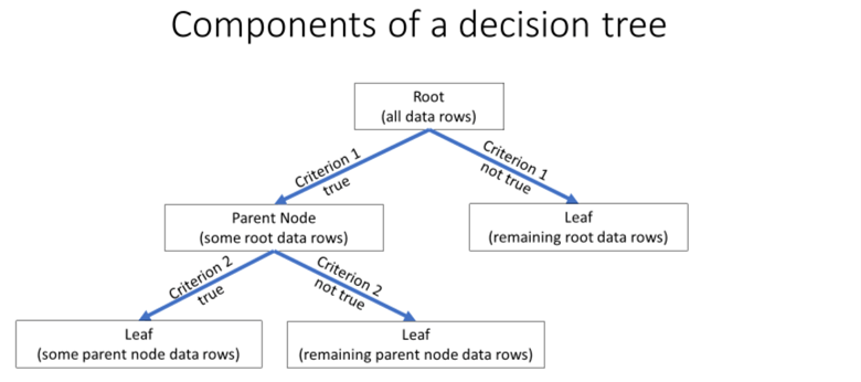
A decision tree model depends on various collections of rows from within a dataset. Sets of rows belong to nodes in the decision tree model. There are three types of nodes in the model. The following screen shot shows the architecture of a decision tree model.
- All data rows initially belong to the root node. The root node has no preceding nodes, but it has two trailing nodes.
- A parent node can contain a subset of data rows. A parent node has
a preceding node and a trailing node. The preceding node can be
- A root node or
- Another parent node
- A leaf node can also contain a subset of rows, but a leaf node has no trailing node.
- Criteria allow for the binary splitting of rows from a root node into a
pair of parent nodes or a parent node and a leaf node. The splitting process
is binary because each criterion can be either true or not true. Rows
belonging to the true outcome go to one node, and rows belonging to the not
true outcome go to another node. The splitting process can proceed until
- a derivative set of rows is composed completely of a single type of row
- a derivative set of rows for a node has a more heterogeneous set of rows than its parent node or
- other special reasons, such as the rows for a derivative node having a minimum count that signals unstable results
The following table shows some arbitrarily composed data that reflects survivor trends by gender and age for the Titanic’s maiden voyage. This is the kind of dataset that the decision tree algorithm is designed to analyze. Each row has an identifier: 1 for a survivor and 0 for not a survivor. In addition, each row has a pair of attribute values: F and M for gender and a number to reflect a passenger’s age.
A common practice is to place women and children in the lifeboats before allowing men to enter lifeboats. The data reflect this practice.
- All survivors either had a gender of F or were M children at or below the age of 10.
- All non-survivors were males above the age of 10 who were not allotted space on a lifeboat.
| Fake Survival Data for Titanic Maiden Voyage | ||
|---|---|---|
| Gender | Age | Survivor (1 = yes, 0 = no) |
| F | 22 | 1 |
| F | 9 | 1 |
| M | 8 | 1 |
| M | 25 | 0 |
| F | 45 | 1 |
| M | 50 | 0 |
| M | 29 | 0 |
| M | 10 | 1 |
| F | 29 | 1 |
To implement a decision tree algorithm, you need to split the root node with all data rows into two groups based on a decision criterion. Then, if one group is pure – made up of only survivors in this sample dataset -- the new derivative node would no longer need to be split. If the other derivative node were not pure, then it is a candidate for a second round of splitting based on a second criterion. You can represent these criteria by a cutoff value for an attribute.
- The gender attribute for the preceding table has just two values – so the appropriate criterion for an attribute is a gender value of F or M.
- The values for the age attribute in this example are continuous. There are multiple ways of specifying splitting criteria for a continuous attribute value. For example, you can inspect the continuous values and discover a good cutoff, such as an age of 10 less. Alternatively, you can bin the continuous values according to some rule, such as at or below the median versus above the median.
Given properly defined attribute cutoff values, you can use any of several different metrics for assessing which is the best criterion for splitting a set of rows. In this tip, each criterion has its own weighted gini score. The criterion with the smallest weighted gini score is the best at splitting the rows in a node. A subsequent section in this tip will demonstrate how to compute weighted gini scores for finding the best criterion for splitting the rows at a node into two groups.
The data for this tip
This tip demonstrates a decision tree algorithm application for grouping states based on weather observations downloaded from the National Oceanic and Atmospheric Administration (NOAA) website. The weather facts are minimum daily temperature in Fahrenheit degrees, inches of daily rain, and inches of daily snow. The weather data are from selected weather stations for the five most populous states based on the 2010 decennial census: California, Florida, Illinois, New York, and Texas. The weather observations come from a previous tip that creates and populates a SQL Server weather data warehouse based on downloaded observations.
There are three steps to preparing the dataset for the decision tree application demonstrated in this tip.
- The weather facts are pulled from the warehouse. The data are grouped by weather station within state and averaged for the three types of weather observations covered by the tip. The dataset contains 24 rows for a selection of 3 to 6 weather stations per state. The columns of the dataset start with state and weather station identifiers that precede three columns with the average of the three types of weather facts for each weather station.
- Next, a median value is computed for each type of weather fact across all 24 weather stations.
- Finally, the average values for each weather station are replaced by bin values denoting whether an average value is at or below versus above the median value for each of the three weather facts. This final transformation of the source data is the dataset used for implementing the decision tree application.
The T-SQL code for performing each of three preceding steps is provided in the download for this tip. The following script shows the code for displaying median-coded bins for each weather station. The data resides in the for_gini_comps_with_meadian_based_bins table. As the name implies, this table contains the source data for computing weighted gini scores. The weighted gini scores indicate which attribute is best for splitting the rows associated with a node in the decision tree.
select *
from dbo.for_gini_comps_with_median_based_bins
order by STATEPROV, noaa_station_id
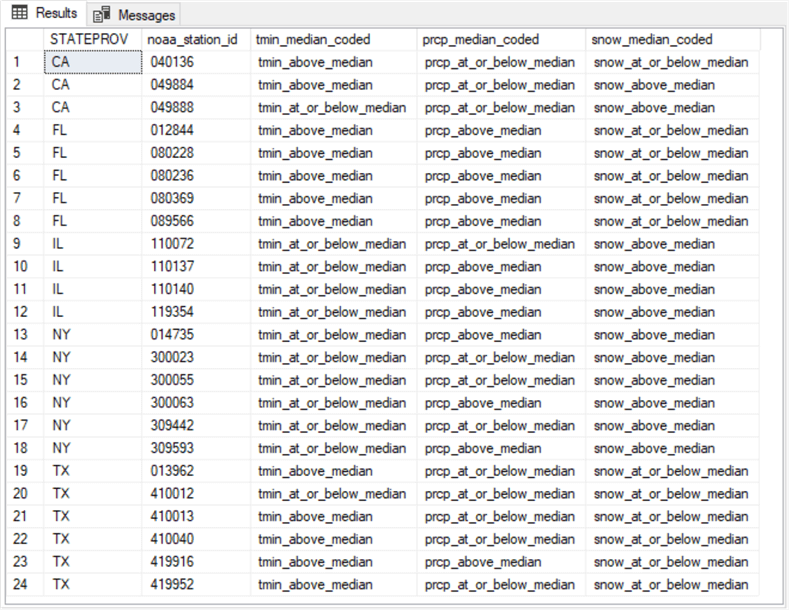
The following screen shot shows the results set from the preceding script.
- The STATEPROV column values are two-character state abbreviations.
- The noaa_station_id column values are six-character fields for identifying weather stations. Each of the 24 rows in the results set has a unique noaa_station_id value. The weather data warehouse contains a facts dimension table for more details besides the station identifier.
- The third, fourth, and fifth columns contain median-coded values, respectively, for minimum daily temperature (tmin), rain (prcp), and snow. Each column value denotes whether the average continuous value for a weather station is at or below the overall median or above the overall median.
Computing gini scores based on the decision tree algorithm
The states from the dataset are split into two parts based on weighted computing gini scores. One part is for NY. The other part is for the remaining states of CA, FL, IL, and TX. There are 6 weather stations in NY, and there is a total of 18 weather stations in the remaining 4 states. The purpose for computing the weighted gini scores is to find which of the three median-coded attributes is the best for distinguishing between NY and the other four states.
Before reviewing the code for the weighted gini scores, this tip shows the inputs and sequence of calculations for computing the tmin weighted gini score. Each branch from a node has its own gini score, and the pair of branches share an overall weighted gini score. The weighted gini score is based on gini scores for each of the two branches from a data node.
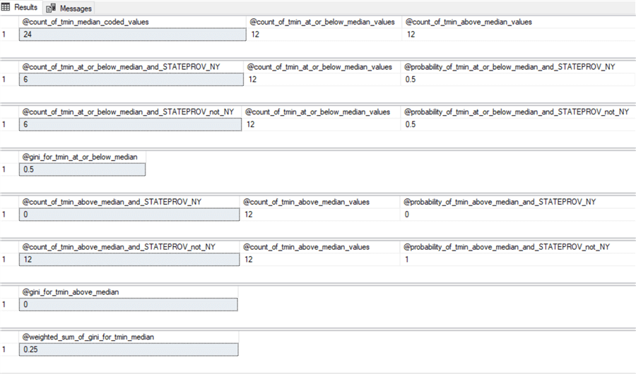
Here is the screen shot with the inputs and the computations for tmin gini scores. These inputs and computations are displayed through a series of eight queries. The screen shot below shows the results set from each of the eight queries.
- The first results set returns three values
- The overall count of dataset rows as @count_of_tmin_median_coded_values
- The count of tmin_median_coded values at or below the median
- The count of tmin_median_coded values above the median
- The second results set also returns three values
- The count of tmin_median_coded values from NY at or below the median
- The count of tmin_median_coded values at or below the median from any state
- The probability of a tmin_median_coded value from NY at or below the median
- The third results set returns the same three types of values for the set of states not including NY.
- The fourth results set returns the gini score for tmin_at_or_below_median values. This gini score equals
1 – (@probability_of_tmin_at_or_below_median_and_STATEPROV_NY2 + @probability_of_tmin_at_or_below_median_and_STATEPROV_not_NY2)
- The fifth, sixth, and seventh results sets display comparable results for the tmin_median_coded values above the median. The seventh results set is computed with the following expression.
1 – (@probability_of_tmin_above_median_and_STATEPROV_NY2 + @probability_of_tmin_above_median_and_STATEPROV_not_NY2)
- The eighth results set returns the weighted tmin_median_code gini score for values at or below the median as well as for values above the median. This value is the overall indicator of the power of tmin_median_coded values for distinguishing rows based on their source – namely, NY or the set of the other four states in the dataset being split. The eighth results set is computed with the following expression. Notice how the expression weights the @gini_for_tmin_at_or_below_median and @gini_for_tmin_above_median values, respectively, by the counts in @count_of_tmin_at_or_below_median_values and @count_of_tmin_above_median_values divided by @count_of_tmin_median_coded_values.
  ((@count_of_tmin_at_or_below_median_values/@count_of_tmin_median_coded_values) * @gini_for_tmin_at_or_below_median)
  +
  ((@count_of_tmin_above_median_values/@count_of_tmin_median_coded_values) * @gini_for_tmin_above_median)
To keep the focus on tmin_median_coded values and their relationships with states, the code for the preceding screen shot starts by creating and populating a table with just three columns -- STATEPROVE, noaa_station_id, and tmin_median_coded. The table’s name is for_gini_comps_tmin_median. Here is the code for achieving this goal.
- The script starts by dropping any prior version of the for_gini_comps_tmin_median table.
- Next, the code creates and populates a fresh version of the for_gini_comps_tmin_median table with the into clause of a query based on the for_gini_comps_with_median_based_bins table.
- The code concludes with a select statement that displays the results set in the for_gini_comps_tmin_median table. The trailing select statement is optional; the statement displays the results set in the for_gini_comps_tmin_median table.
begin try
   drop table dbo.for_gini_comps_tmin_median
end try
begin catch
   print 'for_gini_comps_tmin_median table not available to drop'
end catch

-- list tmin_median_coded with STATEPROV and noaa_station_id identifiers
select STATEPROV, noaa_station_id, tmin_median_coded
into dbo.for_gini_comps_tmin_median
from dbo.for_gini_comps_with_median_based_bins
order by STATEPROV, noaa_station_id

--/*
-- for tutorial purposes only
select *
from dbo.for_gini_comps_tmin_median
order by STATEPROV, noaa_station_id
--*/
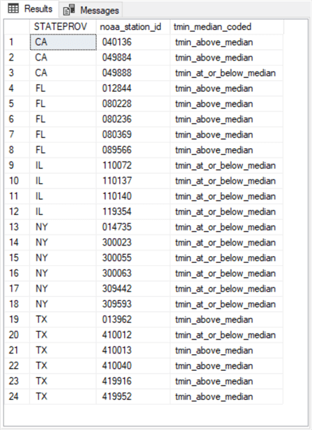
The results set from the preceding script appears below. This results set is the source for the values presented in the preceding screen shot tracing the steps for computing the weighted tmin_median_code gini score for values at or below the median as well as for values above the median.
The following code processes the result set in the preceding screen shot to generate the results sets in the screen shot before the preceding screen shot. The ultimate objective of the code is to compute the weighted gini score for values at or below the median as well as for values above the median. This final quantity appears in the eighth results set in the screen shot before the preceding screen shot. The lower the value of the weighted gini score for an attribute, the better the attribute is at splitting the dataset into two homogeneous groups. A subsequent section demonstrates how to compare the weighted gini scores for each attribute to pick a best attribute for splitting the rows associated with a decision tree node.
- The code for the first results set declares and populates three scalar values.
A single declare variable populates all three local variables. A trailing
select statement displays the local variables.
- The @count_of_tmin_median_coded_values local variable returns the count of all tmin_median_coded values. Although the variable will always hold an integer value, the variable is declared with a float data type. This is because the local variable is subsequently used in divisions where we want to avoid truncation of the quotient. This approach is used widely in the code below for scalar count values.
- The @count_of_tmin_at_or_below_median_values local variable returns the count of all tmin_median_coded values that represent tmin values at or below the median of all tmin values.
- The @count_of_tmin_above_median_values local variable returns the count of all tmin values above the median of all tmin values.
- The trailing select statement displays each of the three local variables declared in section 1.
- The code for the second and third results sets has two declare statements
and two select statements. The code for the second results set is to compute
the probability of tmin values being at or below the median for weather stations
in NY state. The code for the third results set is to compute the probability
of tmin values being at or below the median for weather stations that are not
in NY state (that is, the weather stations from CA, FL, IL, and TX).
- The first declare statement specifies two local variables.
- The @count_of_tmin_at_or_below_median_and_STATEPROV_NY local variable is for the count of rows with NY STATEPROV identifiers that have tmin values at or below the median tmin value across all 24 rows.
- The @count_of_tmin_at_or_below_median_and_STATEPROV_not_NY local variable is for the count of rows with STATEPROV identifiers other than NY that have tmin values at or below the median tmin value across all 24 rows.
- The second declare statement is to compute two different probabilities.
- The @probability_of_tmin_at_or_below_median_and_STATEPROV_NY local variable is to compute the probability of a NY state row having a tmin value at or below the median for all 24 rows.
- The @probability_of_tmin_at_or_below_median_and_STATEPROV_not_NY local variable is to compute the probability of a tmin value at or below the median for all 24 rows when the state is not NY.
- The select statements display the inputs to and the results of the probability
computations for the NY state rows and rows that are not for NY state.
- The first select statement displays the numerator (@count_of_tmin_at_or_below_median_and_STATEPROV_NY) and the denominator (@count_of_tmin_at_or_below_median_values) of the probability for NY state rows as well as the computed NY state probability value (@probability_of_tmin_at_or_below_median_and_STATEPROV_NY).
- The second select statement displays the numerator (@count_of_tmin_at_or_below_median_and_STATEPROV_not_NY) and the denominator (@count_of_tmin_at_or_below_median_values) of the probability for non-NY state rows as well as the computed non-NY state probability value (@probability_of_tmin_at_or_below_median_and_STATEPROV_not_NY).
- The first declare statement specifies two local variables.
- The code for the fourth results set includes a declare statement for a local variable that returns the gini score for tmin values at or below the overall median value as well as a select statement for displaying the gini score. As you can see, the gini score depends on the probability values from the second and third results sets.
- The code for the fifth and sixth results sets has two declare statements
and two select statements. The code for the fifth results set is to compute
the probability of tmin values being above the median for weather stations in
NY state. The code for the sixth results set is to compute the probability
of tmin values being above the median for weather stations that are not in NY
state.
- The first declare statement specifies two local variables for count
values.
- The @count_of_tmin_above_median_and_STATEPROV_NY local variable is for the count of rows with NY STATEPROV identifiers that have tmin values above the median tmin value across all 24 rows.
- The @count_of_tmin_above_median_and_STATEPROV_not_NY local variable is for the count of rows with STATEPROV identifiers other than NY that have tmin values above the median tmin value across all 24 rows.
- The second declare statement is to compute two local variables for probabilities.
- The @probability_of_tmin_above_median_and_STATEPROV_NY local variable is to compute the probability of a NY state row having a tmin value above the median for all 24 rows.
- The @probability_of_tmin_above_median_and_STATEPROV_not_NY local variable is to compute the probability of a tmin value above the median when the state is not NY.
- The first declare statement specifies two local variables for count
values.
- The code for the seventh and eighth results sets includes a pair of declare
statements and a pair of select statements.
- The first declare statement is for a local variable (@gini_for_tmin_above_median) that returns the gini score for tmin values above the overall median value.
- The first select statement is for displaying the @gini_for_tmin_above_median gini score. As you can see, the gini score depends on the probability values from the fifth and sixth results sets.
- The second declare statement is for a local variable (@weighted_sum_of_gini_for_tmin_median) that returns the weighted gini score for tmin values at or below as well as above the overall median value. The expression in the declare statement shows the @weighted_sum_of_gini_for_tmin_median local variable depends on two previously computed gini scores (@gini_for_tmin_at_or_below_median and @gini_for_tmin_above_median) that are weighted by the relative sample size for computing each gini score.
- The second select statement is for displaying the @weighted_sum_of_gini_for_tmin_median local variable value.
-- code for section 1 results set
declare
 @count_of_tmin_median_coded_values float =
(select count(tmin_median_coded) [count_of_tmin_median_coded values]
from dbo.for_gini_comps_tmin_median)

,@count_of_tmin_at_or_below_median_values float =
(select count(tmin_median_coded) [count_of_tmin_at_or_below_median values]
from dbo.for_gini_comps_tmin_median
where tmin_median_coded = 'tmin_at_or_below_median')

,@count_of_tmin_above_median_values float =
(select count(tmin_median_coded) [count_of_tmin_above_median values]
from dbo.for_gini_comps_tmin_median
where tmin_median_coded = 'tmin_above_median')

select
 @count_of_tmin_median_coded_values [@count_of_tmin_median_coded_values]
,@count_of_tmin_at_or_below_median_values [@count_of_tmin_at_or_below_median_values]
,@count_of_tmin_above_median_values [@count_of_tmin_above_median_values]

---------------------------------------------------------------------------------------------------

-- code for section 2 and 3 results sets
declare
@count_of_tmin_at_or_below_median_and_STATEPROV_NY float =
(select count(*) [count of tmin_median_coded = 'tmin_at_or_below_median' and STATEPROV = 'NY']
from dbo.for_gini_comps_tmin_median
where tmin_median_coded = 'tmin_at_or_below_median' and STATEPROV = 'NY')

,@count_of_tmin_at_or_below_median_and_STATEPROV_not_NY float =
 (select count(*) [count of tmin_median_coded = 'tmin_at_or_below_median' and STATEPROV != 'NY']
from dbo.for_gini_comps_tmin_median
where tmin_median_coded = 'tmin_at_or_below_median' and STATEPROV != 'NY')

declare
 @probability_of_tmin_at_or_below_median_and_STATEPROV_NY float =
 (select @count_of_tmin_at_or_below_median_and_STATEPROV_NY
  /
  @count_of_tmin_at_or_below_median_values)
,@probability_of_tmin_at_or_below_median_and_STATEPROV_not_NY float =
 (select @count_of_tmin_at_or_below_median_and_STATEPROV_not_NY
  /
  @count_of_tmin_at_or_below_median_values )


select
 @count_of_tmin_at_or_below_median_and_STATEPROV_NY [@count_of_tmin_at_or_below_median_and_STATEPROV_NY]
,@count_of_tmin_at_or_below_median_values [@count_of_tmin_at_or_below_median_values]
,@probability_of_tmin_at_or_below_median_and_STATEPROV_NY [@probability_of_tmin_at_or_below_median_and_STATEPROV_NY]


select
 @count_of_tmin_at_or_below_median_and_STATEPROV_not_NY [@count_of_tmin_at_or_below_median_and_STATEPROV_not_NY]
,@count_of_tmin_at_or_below_median_values [@count_of_tmin_at_or_below_median_values]
,@probability_of_tmin_at_or_below_median_and_STATEPROV_not_NY [@probability_of_tmin_at_or_below_median_and_STATEPROV_not_NY]

---------------------------------------------------------------------------------------------------

-- code for section 4 results set
declare
 @gini_for_tmin_at_or_below_median float =
  1 -(power(@probability_of_tmin_at_or_below_median_and_STATEPROV_NY,2)
   + power(@probability_of_tmin_at_or_below_median_and_STATEPROV_not_NY,2))


select @gini_for_tmin_at_or_below_median [@gini_for_tmin_at_or_below_median]

---------------------------------------------------------------------------------------------------

-- code for section 5 and 6 results sets
declare
@count_of_tmin_above_median_and_STATEPROV_NY float =
(select count(*) [count of tmin_median_coded = 'tmin_above_median' and STATEPROV = 'NY']
from dbo.for_gini_comps_tmin_median
where tmin_median_coded = 'tmin_above_median' and STATEPROV = 'NY')

,@count_of_tmin_above_median_and_STATEPROV_not_NY float =
 (select count(*) [count of tmin_median_coded = 'tmin_above_median' and STATEPROV != 'NY']
from dbo.for_gini_comps_tmin_median
where tmin_median_coded = 'tmin_above_median' and STATEPROV != 'NY')

declare
 @probability_of_tmin_above_median_and_STATEPROV_NY float =
 (select @count_of_tmin_above_median_and_STATEPROV_NY
  /
  @count_of_tmin_above_median_values)
,@probability_of_tmin_above_median_and_STATEPROV_not_NY float =
 (select @count_of_tmin_above_median_and_STATEPROV_not_NY
  /
  @count_of_tmin_above_median_values )

select
 @count_of_tmin_above_median_and_STATEPROV_NY [@count_of_tmin_above_median_and_STATEPROV_NY]
,@count_of_tmin_above_median_values [@count_of_tmin_above_median_values]
,@probability_of_tmin_above_median_and_STATEPROV_NY [@probability_of_tmin_above_median_and_STATEPROV_NY]

select
 @count_of_tmin_above_median_and_STATEPROV_not_NY [@count_of_tmin_above_median_and_STATEPROV_not_NY]
,@count_of_tmin_above_median_values [@count_of_tmin_above_median_values]
,@probability_of_tmin_above_median_and_STATEPROV_not_NY [@probability_of_tmin_above_median_and_STATEPROV_not_NY]

---------------------------------------------------------------------------------------------------

-- code for section 7 and 8 results sets
declare
 @gini_for_tmin_above_median float =
  1 -(power(@probability_of_tmin_above_median_and_STATEPROV_NY,2) + power(@probability_of_tmin_above_median_and_STATEPROV_not_NY,2))

declare
 @weighted_sum_of_gini_for_tmin_median float =
 ((@count_of_tmin_at_or_below_median_values/@count_of_tmin_median_coded_values) * @gini_for_tmin_at_or_below_median)
  +
 ((@count_of_tmin_above_median_values/@count_of_tmin_median_coded_values) * @gini_for_tmin_above_median)


select @gini_for_tmin_above_median [@gini_for_tmin_above_median]

select @weighted_sum_of_gini_for_tmin_median [@weighted_sum_of_gini_for_tmin_median]
The code for computing weighted gini scores for prcp and snow facts are in the download file. Except for name changes based on the type of weather fact for which a weighted gini score is being computed, the declare and select statements as well as the order of the results sets are the same. However, there is one somewhat significant difference. The above script arranges declare statements with matching select statements in order after one another by results set. The generally corresponding code in the download file starts out by declaring all the local variables, and then follows the declare statements with the select statements for displaying the local variables and their inputs.
Interpreting weighted gini scores and displaying a decision tree
The following table presents the weighted gini scores for tmin_median_coded values, prcp_median_coded values, and snow_median_coded values. Recall that the smaller the weighted gini score for an attribute, the better the attribute is at splitting the rows associated within a node into homogeneous groups. By this rule, the tmin and snow attributes are most effective at splitting NY state rows from the rows for the remaining states. This is because the weighted gini score for tmin and snow attributes (.25) is smaller than the weighted gini score for the prcp attribute (.375).
| Type of median_coded values | Weighted gini score |
|---|---|
| tmin | 0.25 |
| prcp | 0.375 |
| snow | 0.25 |
If you examine some of the values computed on the way to deriving weighted gini scores, you can gain further insights into why tmin and snow attributes are best at splitting rows from NY state from rows for the remaining states.
- For example, six NY state rows have tmin_median_coded values at or below
the median tmin value for rows from all states.
- It is colder in NY on an average daily basis than for the set of other states, including CA, FL, IL, and TX.
- Additionally, because all 6 rows from NY state are in a single group, there is no way to improve the split by supplementing the split based on the tmin attributed with another attribute.
- The snow attribute also results in a perfect split of NY state rows from
the rows for the remaining states. That is, all 6 NY state rows have average
daily snow inches that is greater than the median for the 24 rows for all states.
- Because all 6 rows from NY are classified as snowier than the set of the remaining states, there is no way to improve upon this split.
- In fact, you can use either tmin_median_coded values or snow_median_coded values to split perfectly the NY rows from the rows for the remaining states.
- With respect to the prcp attribute, NY rows and the rows for the remaining
states split evenly.
- That is, 3 of 6 NY rows, or 50%, have average daily precipitation that is at or below the median of all states.
- Similarly, 9 of 18 rows, or 50%, for the other four states have average daily precipitation that is at or below the median of all states.
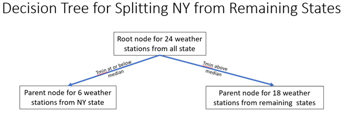
The following screen shot presents a decision tree diagram for the split of the NY state weather stations from the weather stations for the remaining states. The ease of reviewing the results from the decision tree diagram versus the weighted gini scores for attributes is one reason that decision tree models are widely considered easier to understand.
- There are 24 weather stations at the root node for all five states.
- The text for the arrows from the root node to the two leaf nodes below it specifies the criteria for splitting rows into either of the leaf nodes.
- The original set of 24 weather stations can be split into two groups
- 6 weather stations from NY
- 18 weather stations from the remaining states
Next Steps
This tip targets anyone with a basic understanding of T-SQL and an interest in knowing more about the decision tree algorithm for classifying objects as belonging to one of two classes. There are two files in the download or this tip.
- One file in the download contains the source data for the 24 weather stations classified as NY weather stations or weather stations from one of 4 other states (CA, FL, IL, TX). The sample data for this tip includes median coded average values for three attributes per weather station: minimum daily temperature, daily inches of rain, daily inches of snow. The data are available in an .xlsx file.
- The download also contains the T-SQL code for implementing the decision tree algorithm as discussed in this tip.
The decision tree algorithm is a very commonly used data science algorithm for splitting rows from a dataset into one of two groups. Here are two additional references for you to get started learning more about the algorithm.
About the author
 Rick Dobson is an author and an individual trader. He is also a SQL Server professional with decades of T-SQL experience that includes authoring books, running a national seminar practice, working for businesses on finance and healthcare development projects, and serving as a regular contributor to MSSQLTips.com. He has been growing his Python skills for more than the past half decade -- especially for data visualization and ETL tasks with JSON and CSV files. His most recent professional passions include financial time series data and analyses, AI models, and statistics. He believes the proper application of these skills can help traders and investors to make more profitable decisions.
This author pledges the content of this article is based on professional experience and not AI generated.
View all my tips


