Using T-SQL to Quantify Trend Direction and Strength

By: Rick Dobson | Comments | Related: > TSQL

Problem

Is there a way to use multiple sets of moving averages to get estimates of the direction and strength of the trend for underlying data values, such as stock closing prices? Please provide T-SQL code samples for concurrently processing moving averages for multiple different periods and assessing how well the approach works.

Solution

Darryl Guppy may be the most prominent advocate of using multiple moving averages to gain an advantage when trading stocks, commodities, and currencies. He authored several books, is a guest commentator of CNBC Asia, and offers free online resources (here and here) for interpreting multiple moving averages to detect trend direction and strength.

Guppy's analysis framework and techniques are primarily based on relationships between sets of short and long term moving averages. This tip and other preceding tips in this series (for example, here, here, here, and here) demonstrate how to use T-SQL code to implement and apply stock technical indicators like those pioneered by Darryl Guppy for when to buy and sell stocks. This particular tip adapts this web page on how to use multiple moving averages to assess the likely future direction and strength of the trend in a direction.

I emphasize that this is an adaptation and not a verbatim implementation of Guppy's approach.

This is because this tip's goal is to show you how to use T-SQL to assess trend direction and strength. Charts are used in this tip only to clarify the outcome of processing multiple moving averages, but Guppy's approach relies on chart reading techniques for sets of moving averages to anticipate the future direction and strength of moving averages.
Also, this tip leverages resources presented previously in MSSQLTips.com to give you exposure to processing multiple moving averages.

For example, two prior tips (first tip and second tip) make available resources for downloading a SQL Server database named AllNasdaqTickerPricesfrom2014into2017 with historical stock closing prices and exponential moving averages for ten, thirty, fifty, and two hundred periods for stocks listed on the NASDAQ stock exchange.
By leveraging previously computed moving averages for previously downloaded historical price and volume data, this tip aims to expedite your understanding of trend direction and trend strength without distracting you with discussions of how to download historical price and volume data or how to compute exponential moving averages for historical price data.

What do we mean by trend direction and trend strength?

This tip defines trend direction by comparing the moving averages for ten, thirty, fifty, and two hundred periods. When each shorter period moving average is greater than each successively longer period moving average, then the trend direction is defined as up. There are three comparisons for the set of four moving averages available within the AllNasdaqTickerPricesfrom2014into2017 database.

The ten-period moving average must be greater than the thirty-period moving average.
The thirty-period moving average must be greater than the fifty-period moving average
The fifty-period moving average must be greater than the two-hundred-period moving average.

For a trend to exist, these moving average relationships must persist over at least a couple of time series values. Of course, trends are more significant when they extend over many time series values. Each trend must have a distinct starting point, a distinct ending point, and a succession of zero or more time series values between the trend up start and end.

Guppy's prior research indicates that as the moving average values fan out from one another, the strength of a trend up grows. Furthermore, when moving averages converge towards one another, a change may be imminent. The change can be another round of increasing closing prices or the end of a trend up. For example, if the ten-period moving average value falls toward and then below one of the other moving averages, the trend up ceases.

This tip considers the trend up in effect for as long as its three defining relationships hold. It does not matter by how much the shorter moving averages exceed successively longer moving averages. However, the strength of the trend up does depend on the gap between the moving averages. The greater the gap between the moving averages, the stronger the trend up. Greater trend up strength is associated with increasing underlying time series values. Therefore, the largest trend up strength values should be for the largest closing price values.

This tip uses the ratio of the population variance of the moving averages to the average of the moving averages to quantitatively represent trend strength at a point in time.

The average is merely the sum of the moving averages divided by the number of moving averages at a point in time.
The population variance is the average of squared deviations of the moving averages from their average value at a point in time.
The ratio of the two quantities normalizes the population variance of the moving averages relative to the average of the moving averages.

Picking stocks for which to assess trend up and trend strength

As mentioned in the Solution section, the stocks for this examination of trend direction and trend strength are derived from the AllNasdaqTickerPricesfrom2014into2017 database. The code for pulling historical price and volume data for the database from the Yahoo Finance site is available from this tip. This next tip includes a link for downloading a backup file for the database that you can restore in your SQL Server instance. The database contains tables with historical price and volume data for NASDAQ listed stock symbols. You can download from this third tip, a script for computing and saving exponential moving averages for the historical close price data in the database. Running the code for computing exponential moving averages will equip your copy of the AllNasdaqTickerPricesfrom2014into2017 database with a table of exponential moving averages for close prices.

It is the values in the table of exponential moving averages that are analyzed within this tip. The following screen shot displays an Object Explorer view of the columns in the ewma_10_30_50_200 table.

Each row uniquely identifies a set of values for a security by symbol and date values.

The symbol column contains the stock symbol.
The date column denotes the trading date for which the rest of the columns in the row report data.

The close column contains that price at the end of the trading date.
The ewma_10, ewma_30, ewma_50, and ewma_200 columns contain the exponential moving averages, respectively, for ten, thirty, fifty, and two hundred periods. See this tip if you are interested in learning the details for one approach on how to compute exponential moving averages.

There are 3266 distinct stock symbols in the database, but only a small sample of these symbols are suitable for this investigation of trend direction and strength. The primary filtering objective is to find investment grade stocks with substantial amounts of historical data. The following four criteria discovers a total of 245 stocks that meet all criteria for investment grade securities listed on the NASDAQ exchange. The result set is ordered by the difference between the maximum and minimum close prices for historical close prices within each symbol, and each symbol is assigned a row number. The 122 symbols with even row numbers are selected for testing the trend direction and strength code. This approach reserves an additional 123 symbols that you can use to test the code with different symbols than those reported on in this tip.

The criteria for investment grade securities are briefly described below.

Each stock symbol must have a minimum number of daily traded shares of 100,000. This requirement is to ensure that selected stocks are easily traded.
Each stock was required to have data for a minimum of 900 trading days. This ensured that each stock symbol had plenty of data for which to contrast multiple sets of moving averages.
All stock symbols must have their most recent trading day on either November 7 or 8, 2017. The data were collected from Yahoo Finance while updates for the current day of trading (November 8, 2017) were still in progress. So, the last trading day could be November 7 or 8, 2018. If a stock does not have historical data for neither of these two days, then it is not regularly traded on a daily basis, and the stock is excluded from consideration for this tip.
The minimum close price for a stock symbol must be at least $5. Institutional investors, which control the bulk of share transactions, tend to avoid stocks with a share price below $5.

Here's the code to derive and display a sample of 122 symbols with even row numbers. As the code shows, the selected set of symbols are saved in the ##symbol global temporary table.

begin try
drop table ##symbol
end try
begin catch
print '##symbol not available to drop'
end catch

-- put symbol list into ##symbol
select 
* 
into ##symbol
from
(
-- returns half of 245 symbols
-- returns symbols with 
--		odd row_number values when row_number % 2 = 1
--		even row_number values when row_number % 2 = 0
select *
from
(
-- set of symbols with 
--		minimum volume > 100000
--		most recent date of '2017-11-07' or '2017-11-08'
--		at least 900 time series rows of data
--		minimum close price of $5
-- 245 symbols meet the criteria
-- row_number order is desc on max_close-min_close
select 
row_number() over (order by max_close-min_close desc) row_number, *
from
(
-- 3266
select
 symbol
,min([close]) min_close
,max([close])  max_close
,min(volume)  min_volume
,min(date)    min_date
,max(date)    max_date
,count(*)     number_recs
FROM [AllNasdaqTickerPricesfrom2014into2017].[dbo].Results_with_extracted_casted_values
group by symbol
) for_outer_query
where 
min_volume > 100000
and max_date >= '2017-11-07'
and number_recs > 900
and min_close > 5
) for_odd_even_row_number

where (row_number % 2) != 1
) for_even_row_sample

-- display sample symbols
select * from ##symbol order by row_number

Code to discover start and end dates for trend up cycles

As noted above each trend must have at least two time series values -- a start date and an end date. The overwhelming majority of trend cycles have many more than two time series values. The following script discovers the start and end dates for the sample of symbols in the ##symbol table. For the sample of 122 symbols, there are a total of 1260 trend up cycles. The code copies the symbol along with the start and end dates for each trend up cycle and a trend up indicator (trend_10_200_up) into the ##mma_trend_up_starts_and_ends table. A commented select statement at the bottom script can display the column values of each of the trend up cycles.

There are two core parts to the script. These core parts reside in the for_start_end subquery. The first core part finds trend up start dates, and the second part searches for trend up end dates. The criteria for a start date row and end date row are distinctly different. There are three criteria for each type of row.

The start date row criteria are these.

The current row must have its ten-period moving average value greater than its thirty-period moving average, and its thirty-period moving average greater than its fifty-period moving average, and its fifty-period moving average greater than its two-hundred-period moving average. A T-SQL sign function evaluates compliance with each component of the criterion. This criterion's value, which is the sum of the three sign functions, is in a column named trend_10_200_up. The sum of the three sign functions must equal three to meet the criterion's requirement.
A second criterion examines the trend_10_200_up expression outcome for the row preceding the current row. A lag function with a lag of one can specify this column value. The trend_10_200_up expression outcome must not equal three otherwise the current row would not be a start row for a trend up cycle. This criterion's value is in a column named trend_10_200_up_lag1.
The third criterion examines the trend_10_200_up expression outcome for the row after the current row. The lead function with a lead of one can specify this column value. The trend_10_200_up expression outcome must equal three otherwise the current row would not be a start row for a trend up. Recall that a trend up cycle must be defined by at least two contiguous trading dates that trend in an upward direction. This criterion's value is retained in a column named trend_10_200_up_lead1.

The end date row criteria are these. The criteria values populate the same three columns of the for_start_end subquery, and the criteria use the same basic expressions. However, end row criteria require a different pattern of expression values than the start row criteria.

The current row expression value which populates the trend_10_200_up column must equal three because the end row is part of the trend up cycle, and the trend up is defined by each shorter period moving average exceeding its successively longer period moving average.
The preceding row for the current row which populates the trend_10_200_up_lag1 column in the for_start_end subquery must also equal three. This preceding row is necessarily part of the trend up series of moving averages.
The row following the current row which populates the trend_10_200_up_lead1 column in the for_start_end subquery must not equal three. This criterion value actually defines a termination to the trend up.

Aside from the symbol and date columns and the trend_10_200_up, trend_10_200_up_lag1, and the trend_10_200_up_lead1 columns, there is one more column in the for_start_end subquery. The row_type column has one of two distinct values. The body of the for_start_end subquery concatenates the end rows behind the start rows. The row_type column value allows the script to separately identify start rows from end rows in the concatenated for_start_end subquery result set.

The row_type value is "start" for start rows.
The row_type value is "end" for end rows.

The for_start_end subquery is nested within another subquery named for_excluding_rows. This outer subquery groups for_start_end subquery result set rows by symbol, date, trend_10_200_up, trend_10_200_up_lag1, and trend_10_200_up_lead1, and it marks rows for exclusion by a subsequently specified filter. These grouped row values are processed by a case statement that assigns a value to the marked_row_to_delete column. When the last row in the result set sorted by date_start has a "start" value for row_type, then "delete" is assigned to marked_row_to_delete column. Otherwise, the marked_row_to_delete column implicitly has a null column value.

The next outer subquery named starts_and_ends filters the for_excluding_rows result set to retain just those rows with marked_row_to_delete column values of null. This filtering process excludes the last row in the for_excluding_rows result set if that row has a "start" value for row_type. The exclusion is required because trailing rows with a "start" row_type do not ever end their trend up cycle within the context of the sample data. This is because the trend up extends beyond the end of the data in the source time series data.

The code within the start_and_ends subquery identifies separate start and end rows for each trend up cycle in its result set. The output from the starts_and_ends subquery is a set of paired rows with the first row containing the start date for a cycle and the second row containing the end date for a cycle. However, two remaining queries re-shape the result set so that there is a single row for each cycle with separate columns for the start date and end date of each trend up cycle.

The starts_and_ends_on_single_rows subquery uses a lead function to incorporate the end date value into the start row for trend up cycles.
Next, the outermost query, for_single_row_result_set, excludes the end rows from the result set with a where clause filter so that there is just one row per trend up cycle with both start and end date column values. The outermost query in combination with a try…catch block also copies its result set into a fresh copy of the ##mma_trend_up_starts_and_ends table.

use AllNasdaqTickerPricesfrom2014into2017
go

-- start and end rows for trend up
-- multiple moving average cycles

begin try
drop table ##mma_trend_up_starts_and_ends
end try
begin catch
print '##mma_trend_up_starts_and_ends not available to drop'
end catch

select 
symbol
,date_start
,date_end
,trend_10_200_up
into ##mma_trend_up_starts_and_ends
from
(
-- for final single_row result set
select 
symbol
,date date_start
,lead(date,1) over (partition by symbol order by date) date_end
,trend_10_200_up
,trend_10_200_up_lag1
,trend_10_200_up_lead1
,row_type
,marked_row_to_delete
from
(
-- get start dates with row_type
-- for deleting incomplete cycles
select 
symbol
,date
,trend_10_200_up
,trend_10_200_up_lag1
,trend_10_200_up_lead1
,row_type
,marked_row_to_delete
from
(
select 
symbol
,date
,trend_10_200_up
,trend_10_200_up_lag1
,trend_10_200_up_lead1
,row_type
,
case
	when max(date) over (partition by symbol order by symbol) = date
		and row_type = 'start' then 'delete'
end marked_row_to_delete
from
(
-- get start dates
select 
symbol
,date
,trend_10_200_up
,trend_10_200_up_lag1
,trend_10_200_up_lead1
,'start' row_type
from
(
-- get history of trend_10_200_up for stocks in ##symbol
select 
symbol, date, [close], ewma_10, ewma_30, ewma_50, ewma_200
,
(SIGN(ewma_10 - ewma_30)
+
SIGN(ewma_30 - ewma_50)
+
SIGN(ewma_50 - ewma_200)
) trend_10_200_up
,
case
	when symbol = lag(symbol,1) over (partition by symbol order by symbol)
	then
	lag
	(
	(SIGN(ewma_10 - ewma_30)
	+
	SIGN(ewma_30 - ewma_50)
	+
	SIGN(ewma_50 - ewma_200)
	)
	,1
	) over (partition by symbol order by date) 
end trend_10_200_up_lag1
,
case
	when symbol = lead(symbol,1) over (partition by symbol order by symbol)
	then
	lead
	(
	(SIGN(ewma_10 - ewma_30)
	+
	SIGN(ewma_30 - ewma_50)
	+
	SIGN(ewma_50 - ewma_200)
	)
	,1
	) over (partition by symbol order by date) 
end trend_10_200_up_lead1
from ewma_10_30_50_200
where symbol in (select symbol from ##symbol)
group by symbol, date, [close], ewma_10, ewma_30, ewma_50, ewma_200
) for_start_end
group by symbol, date, trend_10_200_up, trend_10_200_up_lag1, trend_10_200_up_lead1
having 
trend_10_200_up = 3
and 
trend_10_200_up_lag1 !=3
and
trend_10_200_up_lead1 =3

union

-- get end dates
select 
symbol
,date
,trend_10_200_up
,trend_10_200_up_lag1
,trend_10_200_up_lead1
,'end' row_type
from
(
-- get history of trend_10_200_up for stocks in ##symbol
select 
symbol, date, [close], ewma_10, ewma_30, ewma_50, ewma_200
,
(SIGN(ewma_10 - ewma_30)
+
SIGN(ewma_30 - ewma_50)
+
SIGN(ewma_50 - ewma_200)
) trend_10_200_up
,
case
	when symbol = lag(symbol,1) over (partition by symbol order by symbol)
	then
	lag
	(
	(SIGN(ewma_10 - ewma_30)
	+
	SIGN(ewma_30 - ewma_50)
	+
	SIGN(ewma_50 - ewma_200)
	)
	,1
	) over (partition by symbol order by date) 
end trend_10_200_up_lag1
,
case
	when symbol = lead(symbol,1) over (partition by symbol order by symbol)
	then
	lead
	(
	(SIGN(ewma_10 - ewma_30)
	+
	SIGN(ewma_30 - ewma_50)
	+
	SIGN(ewma_50 - ewma_200)
	)
	,1
	) over (partition by symbol order by date) 
end trend_10_200_up_lead1
from ewma_10_30_50_200
where symbol in (select symbol from ##symbol)
group by symbol, date, [close], ewma_10, ewma_30, ewma_50, ewma_200
) for_start_end
group by symbol, date, trend_10_200_up, trend_10_200_up_lag1, trend_10_200_up_lead1

having 
trend_10_200_up = 3
and 
trend_10_200_up_lag1 =3
and
trend_10_200_up_lead1 !=3
) for_excluding_rows
) starts_and_ends
where marked_row_to_delete is null
) starts_and_ends_on_single_rows
) for_single_row_result_set

where row_type = 'start'

order by symbol, date_start

-- returns 1260 trend up cycles for 122 symbols
-- select * from ##mma_trend_up_starts_and_ends

Code to compute trend strength

After computing the start and end dates for trend up cycles for stock symbols, it is of value to estimate the trend strength. Not all trend up cycles are equally strong, and even the same cycle can have its strength grow, consolidate or even weaken, and grow again before ultimately declining so that the trend ceases. It is important to know trend strength because

close prices rise when strength increases
close prices decline when strength decreases

Computing trend strength is relatively easy. You compute trend strength for individual trading days.

First, you need to compute the average of the moving averages on a trading day.
Next, you can use the average of the square deviations of the moving averages on a day from their average value for that day to compute the population variance for the day.
Finally, you compute the trend strength on a day as the ratio of the population variance divided by the average.

The following T-SQL script implements the preceding steps for computing trend strength. The code's design relies on nested queries. To keep the focus on the computation, the script computes the trend strength values for each trading day whether or not it is in a trend up cycle.

The innermost subquery named ewmas_with_avg computes the average of the ten, thirty, fifty, and two hundred period moving averages on a day.

The source for this subquery is the ewma_10_30_50_200 table from the AllNasdaqTickerPricesfrom2014into2017.
Because these values are not saved in a normalized format, it is not possible to use the avg function to compute the daily average of a column of exponential moving averages for a symbol.
However, it is a trivial matter to take the sum of the four exponential moving averages on each trading day and divide by four.
The column names for the result set from the innermost query are: symbol, date, close, ewma_10, ewma_30, ewma_50, ewma_200, and avg_ewma.

The second level query named ewmas_with_avg_var computes the population variance for the moving averages on a trading day.

The source for this subquery is the result set from the innermost query.
As with the avg function, you cannot use the SQL Server var function on a column of exponential moving average values because the exponential moving averages are in de-normalized format.
However, as covered in this reference source, the population variance, such as for the four exponential moving averages on a trading day, is merely the sum of the squared deviations of the individual values from their average value divided by the number of population values. This is another expression for the average squared deviations of the moving averages from their mean moving average.
The code in the second level query shows how to use the T-SQL power function to return a squared deviation value. The T-SQL ^ operator does not work for currency data type values, but the T-SQL power function does.

The outermost query performs three major functions.

This query derives its input from the result set of the second level query. As a result, it has access to the average and population variance values for the exponential moving averages on each trading day.
The three major functions are as follow.

It computes trend strength (var_div_avg) as the population variance of the exponential moving averages on each trading day divided by the average of the exponential moving averages on each trading day.
It forms a result set with these columns: symbol, date, close, avg_ewma, variance, and var_div_avg.
In combination with a try…catch block at the top of the script, the outermost query creates and populates a table (##ratio_of_variance_to_mean_with_close) with strength values (var_div_avg) for each trading date in the ewma_10_30_50_200 table.

-- code for ##ratio_of_variance_to_mean_with_close

use AllNasdaqTickerPricesfrom2014into2017
go

-- create and populate ##ratio_of_variance_to_mean_with_close

begin try
drop table ##ratio_of_variance_to_mean_with_close
end try
begin catch
print '##ratio_of_variance_to_mean_with_close not available to drop'
end catch

select 
 symbol
,date
,[close]
,avg_ewma
,variance
,variance/avg_ewma var_div_avg
into ##ratio_of_variance_to_mean_with_close
from
(
-- all exponential moving averages
-- for symbols in ##symbol with the
-- average of exponential moving averages
-- and variance of exponential moving averages 
-- per trading date
select
 symbol
,date
,[close]
,ewma_10
,ewma_30
,ewma_50
,ewma_200
,avg_ewma
,
(
power((ewma_10 - avg_ewma),2)
+
power((ewma_30 - avg_ewma),2)
+
power((ewma_50 - avg_ewma),2)
+
power((ewma_200 - avg_ewma),2)
)/4 variance
from
(
-- all exponential moving averages
-- for symbols in ##symbol with the
-- average of exponential moving averages
-- per trading date
select 
 symbol
,date
,[close]
,ewma_10
,ewma_30
,ewma_50
,ewma_200
,(ewma_10+ewma_30+ewma_50+ewma_200)/4 avg_ewma
from ewma_10_30_50_200
where symbol in (select symbol from ##symbol)
) ewmas_with_avg
) ewmas_with_avg_var
order by symbol, date

-- optionally, remove comment marker for next line to display strength
-- select * from ##ratio_of_variance_to_mean_with_close

To use the trend strength values from the ##ratio_of_variance_to_mean_with_close table within the context of trend up cycles, the trend strength values need to be joined to the values in the ##mma_trend_up_starts_and_ends table. This join will permit you to correlate the trend strength values to the close price values within trend up cycles. Recall that the ##mma_trend_up_starts_and_ends table has start and end dates for trend up cycles. For the sample of 122 stock symbols, there are 1260 trend up cycles. By joining the ##mma_trend_up_starts_and_ends table with the ##ratio_of_variance_to_mean_with_close table, you will end up with a result set that has trend strength and close price for each trading day within each trend up cycle.

The following script demonstrates how to implement the join with a left join of the ##ratio_of_variance_to_mean_with_close table to the ##mma_trend_up_starts_and_ends table.

The single_row_source subquery references the ##mma_trend_up_starts_and_ends table in its from clause. This subquery uses a row_number function with a cycle_in_symbol column name to assign numbers to the sequential trend up cycles for each symbol. The single_row_source subquery result set contains a single row for each trend up cycle across all 122 stock symbols in the sample.
The var_ratio subquery result set contains a single row for each row in the ##ratio_of_variance_to_mean_with_close table which aligns with each row in the underlying ewma_10_30_50_200 table within the AllNasdaqTickerPricesfrom2014into2017 database. There are three criteria for the left join in the on clause.

First, the two row sources must match by symbol.
Next, the date column value from the var_ratio result set must be greater than or equal to the start_date for a matching trend up cycle from the single_row_source result set.
Additionally, the date column value from the var_ratio result set (date_from_var_ratio) must be less than or equal to the end_date for a matching trend up cycle from the single_row_source result set.

The outer query for the two subqueries identifies each row by symbol_from_single_row_source, cycle_in_symbol, date_start, date_end, and date_from_var_ratio. In addition to these identification column values, the strength value (var_div_avg_from_var_ratio) and close price (close_from_var_ratio) for each trading day appear on each row of the outermost query's result set.
Finally, an order by clause sorts rows by symbol_from_single_row_source and date_start from the single_row_source result set, and date_from_var_ratio from the var_ratio result set.

-- data for strength vs close price
select 
 symbol_from_single_row_source
,cycle_in_symbol
,date_start
,date_end
,date_from_var_ratio
,var_div_avg_from_var_ratio
,close_from_var_ratio 
from
(
select 
 row_number() over (partition by symbol order by symbol) cycle_in_symbol
,symbol symbol_from_single_row_source
,date_start
,date_end
,trend_10_200_up 
from ##mma_trend_up_starts_and_ends
) single_row_source

left join

(
select 
 symbol symbol_from_var_ratio
,[date] date_from_var_ratio 
,[close] close_from_var_ratio 
,avg_ewma avg_ewma_from_var_ratio  
,variance variance_from_var_ratio 
,var_div_avg var_div_avg_from_var_ratio
from ##ratio_of_variance_to_mean_with_close 
) var_ratio

on 
single_row_source.symbol_from_single_row_source = var_ratio.symbol_from_var_ratio
and var_ratio.date_from_var_ratio >= single_row_source.date_start
and var_ratio.date_from_var_ratio <= single_row_source.date_end

order by symbol_from_single_row_source, date_start, date_from_var_ratio

Does trend strength correlate with close prices within trend up cycles?

Let me inform you before diving into details that the short answer to the question raised by this section's header is yes. If you want to know more, read the rest of the section.

There are at least two levels for assessing if rising trend strength values correlate with rising close prices. First, you can examine the correlation at the level of stock symbols - namely, for all the trend strength values for a symbol does price go up when trend strength goes up. Second, you can view the association between trend strength values and close prices at the level of individual trend up cycles within a stock symbol. Recall that there are a total of 1260 trend up cycles across the 122 symbols in our sample analysis data. The result set from the preceding query has a trend strength value and a close price for each trading day within each trend cycle for all 122 stock symbols.

In order to explore the correlations between trend strength values and close prices, the "trend strength vs close price" xlsx file was populated with excerpts from the result set for the preceding query. This file is among those available with the download with this tip.

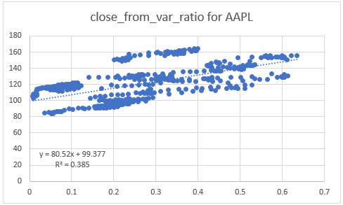
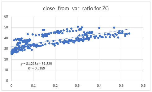
The xlsx file includes data for seven stock symbols. The symbols are: AAPL, AAXN, ACWI, NFLX, NUAN, YY, and ZG. The seven plots below show all the data for each of these symbols. The close prices are along the vertical axis and the trend strength values are along the horizontal axis.

As you can see, larger trend strength values are associated with larger close prices across all seven symbols.

The degree of the correlation as reflected by varying R2 values is not consistent across symbols. For example, the largest coefficient of determination value is .8297 for the ACWI symbol, and the smallest coefficient of determination is .2374 for NFLX. The ACWI symbol is for an exchange traded fund that trades like a stock on the NASDAQ exchange. The NFLX symbol represents NetFlix, Inc., which is an international video production and streaming service.
Also, the slope and intercept values for the fitted regression lines for close prices on trend strength vary substantially across symbols. This is evident from the widely varying slope and intercept values across fitted regression lines for symbols.

At the level of individual trend cycles within a symbol, the degree of correlation between trend strength value and close price was typically much stronger than across all the trend strength values and close prices. The following screen shot displays two plots for the second and third trend up cycles for the AAPL symbol. This symbol represents Apple, Inc. - an international mobile phone and computer manufacturer and marketer. Column B displays which trend up cycle shows in the plot.

Note that the two trend up cycles have a vastly different number of trading days. The second trend up cycle has just four trading days, but the third trend up cycle extends over many more days (the full set of thirty-eight trading days does not fit on the screen shot). It is not unusual for the number of trading days to vary greatly across different cycles within a symbol.
The coefficient of determination for the two plots are, respectively, .9788 and .8906, for the second and third trend up cycles. Both coefficients of determination are well in excess of the coefficient of determination for all AAPL close prices versus trend strength values (.385). Again, it was typical of the other symbols as well for the correlation between trend strength and close price to be greater at the level of individual trend up cycles than across all the cycles within a symbol.

You are invited to view the xlsx file with plots showing data for all seven symbols. There are on average slightly more than ten cycles per symbol. For the seven symbols examined, there was a consistent pattern for rising trend strength values to be associated with rising closing prices within trend up cycles. For just two plots out of slightly more than seventy, the relationship went the other way. For both of the plots with declining close prices for rising trend strength values, there were relatively few data points involved. If you are interested, you can examine the relationships for trend cycles for other symbols by copying values from the result set from the preceding query to the workbook file and creating your own custom plots.

Can maximum trend strength value predict maximum close price?

Before diving into the details, it may be helpful to note that the answer in the section header is yes. In fact, across the 1260 trend up cycles for the 122 stocks in the sample, there is a nearly a perfect correlation between the close price associated with the maximum trend strength value and the maximum close for trend up cycles. This section shows how to generate results with T-SQL to confirm this outcome.

The following pair of scripts perform the task of computing an average close price for the maximum trend strength value in each trend up cycle. This approach guarantees a consistently computed close price for a maximum trend strength value whether there is just one occurrence or more than one occurrence of a maximum trend strength value in a trend up cycle.

The first script computes the maximum trend strength value per trend up cycle and saves it in the #temp table.

The columns in the #temp table identify the trend up cycle and display the maximum trend strength value.

symbol, date_start, and date_end identify the 1260 trend up cycles in our sample
max_var_div_avg is the maximum trend strength value for the cycle identified by the other three column values

As you can see, the code for the first script follows design guidelines for the scripts in the "Code to compute trend strength" section for computing trend strength value. Basically, values from the ##ratio_of_variance_to_mean_with_close table are left joined to values from the ##mma_trend_up_starts_and_ends

A major distinction is the addition of a group by close to group row values by symbol, date_start, date_end, and var_div_avg.
Once the rows are grouped, a max function is used to compute the maximum var_div_avg, which denotes trend strength. Therefore, the max function value represents the maximum trend strength value per trend up cycle.

The second script computes the average close price for each maximum trend strength value.

The #temp table has the maximum trend strength value for each trend up cycle. Therefore, each #temp row is for a different trend up cycle.
The query in the second script right joins the ##ratio_of_variance_to_mean_with_close query result set to the rows of the #temp table. The join makes available the close prices for each trend up cycle.
The outer query of the joined result set for the #temp table with the ##ratio_of_variance_to_mean_with_close table groups rows by #temp.symbol ,#temp.date_start, #temp.date_end, and #temp.max_var_div_avg.
The outer query also uses the avg and count functions to compute the average close price and count of values per maximum trend strength value within a trend up cycle.
Therefore, the outer query makes available the average close price value for maximum trend strength values per trend up cycle. This average close price value can be compared to the maximum close price value per trend up cycle.

-- for comparison of close from max_var_div_avg to max_close
-- by trend_up cycles across 122 symbols with 1260 cycles

begin try
drop table #temp
end try
begin catch
print '#temp not available to drop'
end catch

-- maximum var_div_avg per cycle in symbol cycle
-- with first and max close price values
select 
distinct
symbol
,date_start
,date_end
,max(var_div_avg) over (partition by symbol,date_start order by [date_start]) max_var_div_avg

into #temp
from
(
-- list of var_div_avg and close with
-- trend_up_starts_and_ends
select 
symbol_from_single_row_source symbol
,date_start
,date_end
,trend_10_200_up 
,date_from_var_ratio [date]
,close_from_var_ratio [close]
,avg_ewma_from_var_ratio avg_ewma 
,variance_from_var_ratio variance
,var_div_avg_from_var_ratio var_div_avg
from
(
select 
symbol symbol_from_single_row_source
,date_start
,date_end
,trend_10_200_up 
from ##mma_trend_up_starts_and_ends
) single_row_source

left join

(
select 
symbol symbol_from_var_ratio
,[date] date_from_var_ratio 
,[close] close_from_var_ratio 
,avg_ewma avg_ewma_from_var_ratio  
,variance variance_from_var_ratio 
,var_div_avg var_div_avg_from_var_ratio

from ##ratio_of_variance_to_mean_with_close 
) var_ratio

on 
single_row_source.symbol_from_single_row_source = var_ratio.symbol_from_var_ratio
and var_ratio.date_from_var_ratio >= single_row_source.date_start
and var_ratio.date_from_var_ratio <= single_row_source.date_end
) var_div_avg_and_close_grouped

group by 
symbol
,date_start
,date_end
,var_div_avg

order by var_div_avg_and_close_grouped.symbol, date_start


-- prior query populates #temp with max_var_div_avg
-- by symbol, date_start, date_end

-- this query right joins raw detail for
-- symbol, date, var_div_avg, [close] 
-- from ##ratio_of_variance_to_mean_with_close
-- to #temp fields

-- the result set is grouped by 
-- symbol, date_start, date_end, max_var_div_avg
-- to report avg close price and count of observations
-- per group
select 
 #temp.symbol
,#temp.date_start
,#temp.date_end
,#temp.max_var_div_avg
,avg([close]) [close]
,count(*) obs
from #temp

right join

(
select symbol, date, var_div_avg, [close] 
from ##ratio_of_variance_to_mean_with_close 
) details

on 
details.symbol = #temp.symbol
where
details.date >= #temp.date_start
and details.date <= #temp.date_end
and details.var_div_avg = #temp.max_var_div_avg

group by
 #temp.symbol
,#temp.date_start
,#temp.date_end
,#temp.max_var_div_avg
order by #temp.symbol, #temp.date_start

See below an excerpt of rows from the result set for the preceding pair of scripts. It displays output for the ACWI and ADBE symbols. There are 11 trend up cycles for the ACWI symbol, which represents an exchange traded fund, and 14 trend up cycles for the ADBE symbol, which represents Adobe Systems Incorporated.

The max_var_div_avg column displays the maximum trend strength value for a trend up cycle for a symbol.
The obs column shows the count of maximum trend strength values within each trend up cycle.
The close column presents the average close price for trend strength value(s) within a trend up cycle.

The next script computes the maximum close price per trend up cycle from the left join of the ##ratio_of_variance_to_mean_with_close table with the ##mma_trend_up_starts_and_ends table. Recall that the ##mma_trend_up_starts_and_ends table has symbol, start dates, and end dates for trend up cycles. The ##ratio_of_variance_to_mean_with_close table has close price values for trading days in trend cycles. By taking the max function value of the close price values from the ##ratio_of_variance_to_mean_with_close table, the script computes the maximum close price per trend up cycle from the joined result set. These values are saved in the ##max_close_by_cycle table.

-- max_close by 
-- symbol, date_start, date_end

begin try
drop table ##max_close_by_cycle
end try
begin catch
print '##max_close_by_cycle not available to drop'
end catch

select 
 row_number() over (order by symbol_from_single_row_source, date_start) row_number
,symbol_from_single_row_source symbol
,date_start date_start
,date_end date_end
,max(close_from_var_ratio) max_close
into ##max_close_by_cycle
from
(
select 
symbol symbol_from_single_row_source
,date_start
,date_end
,trend_10_200_up 
from ##mma_trend_up_starts_and_ends
) single_row_source

left join

(
select 
 symbol symbol_from_var_ratio
,[date] date_from_var_ratio 
,[close] close_from_var_ratio 
,avg_ewma avg_ewma_from_var_ratio  
,variance variance_from_var_ratio 
,var_div_avg var_div_avg_from_var_ratio

from ##ratio_of_variance_to_mean_with_close 
) var_ratio

on 
single_row_source.symbol_from_single_row_source = var_ratio.symbol_from_var_ratio
and var_ratio.date_from_var_ratio >= single_row_source.date_start
and var_ratio.date_from_var_ratio <= single_row_source.date_end

group by symbol_from_single_row_source, date_start, date_end

order by symbol, date_start

Here's an excerpt from the rows of the ##max_close_by_cycle table that are for the same symbols and trend up cycles as in the preceding screen shot. Notice that the start date and end date column values are the same between the two output listings. However, the max_close column values from the output below are often the same but sometimes greater than those from the preceding output listing. This is because the max_close column values are for the maximum close price within each trend up cycle, but the close column values are the average close price(s) associated with the maximum trend strength value within each trend up cycle.

The final screen shot for this tip includes the columns from the result set with maximum trend strength values (max_var_div_avg) and the associated average close prices by trend up cycle versus the maximum close prices per trend up cycle. These values are copied to the Predict max_close tab of the "trend strength vs close price" xlsx file; recall this file is available for download with the other files for this tip.

The chart in the screen shot shows the regression for predicting max_close values based on the average close price for max_var_div_avg values.
As you can see, the coefficient of determination is nearly 1 at 0.9997.
In addition, slope is 1.0085. This value is very nearly 1, which means that changes in average close for max_var_div_avg values map nearly identically to changes in max_close values.
Finally, the intercept at .1262 is just slightly more than 0. This means that the close from max_var_div_avg values are just .1262 less on average than the max_close values.

Next Steps

There are three steps necessary for trying out the scripts from this tip.

First, you need to download the AllNasdaqTickerPricesfrom2014into2017 database from this tip. The backup file from the tip includes NASDAQ historical price and volume data.

Next, you need to download and run a script file from this other prior tip on how to create and populate the ewma_10_30_50_200 table for all stocks in the database.

The third step is to download the files for this tip from this link. The link will enable you to compute trend direction and trend strength for a set of stock symbols. You can use the code as is for the symbols reported in this tip or modify the code for populating the ##symbol table to use another set of symbols. Recall that a slight tweak to the code for picking symbols will yield you a fresh sample of 123 symbols. With the fresh sample of symbols, you can personally verify if the relationships demonstrated in this tip are present with another sample of symbols.

Finally, I close by indicating that this tip is not recommending any particular stocks, including those for which results are reported in this tip nor is it recommending any specific trading rules. The stocks reported on in this tip were selected based on precise business rules and the goals of the tip. At the time that I submitted this tip to MSSQLTips.com, I and my family members held positions in a subset of these stocks. I do occasionally use selected technical indicators, including trend direction and trend strength, in making decisions about which stocks to buy and when to sell them, but I do not routinely use the precise trading rules covered in this tip.

About the author

Rick Dobson is an author and an individual trader. He is also a SQL Server professional with decades of T-SQL experience that includes authoring books, running a national seminar practice, working for businesses on finance and healthcare development projects, and serving as a regular contributor to MSSQLTips.com. He has been growing his Python skills for more than the past half decade -- especially for data visualization and ETL tasks with JSON and CSV files. His most recent professional passions include financial time series data and analyses, AI models, and statistics. He believes the proper application of these skills can help traders and investors to make more profitable decisions.

This author pledges the content of this article is based on professional experience and not AI generated.

View all my tips