Relative Strength Index Predictions with SQL Code

By: Rick Dobson | Updated: 2022-06-17 | Comments (3) | Related: > TSQL

Problem

I am a database professional and an aspiring data scientist. I seek data science principles and data management best practices that facilitate the prediction of things like when to buy and sell financial securities. Please present and describe a model implemented with SQL code to predict based on the Relative Strength Index when to buy and sell financial securities. Demonstrate how to select better-performing model parameters.

Solution

The Relative Strength Index (also commonly referred to as the RSI) is widely used by stock market analysts and personal investors who are technically inclined. The tool was initially developed in 1978 by a technical analyst named J. Welles Wilder in a book titled "New Concepts in Technical Trading Systems". Stock market analysts refer to the RSI as a price momentum oscillator. RSI values can oscillate in the range of 0 through 100. A value of 0 indicates no rising price momentum, and a value of 100 indicates maximum price momentum. For stock-based securities, the RSI typically varies from somewhat below 30 through somewhat above 70. When the RSI is 70 or greater it is often called overbought. Likewise, when the RSI is 30 or less, it is often called oversold. Examples of how to use the RSI to decide when to buy and sell securities are abundant (for example, here, here, here, and here).

MSSQLTips.com published two previous tips on the RSI. The first prior tip was a general introduction to the RSI for T-SQL developers. This tip covered some computational issues with T-SQL for the RSI, and it showed some sample RSI results for six ticker symbols over a four-year timeframe from 2014 through 2017. It was a data mining tip that tried to link RSI values to stock prices, but it offered no model on how to predict when to buy and sell dates based on RSI values. The second tip drilled down on the computational process for the RSI with SQL. Furthermore, it offered a more complete comparison of RSI values computed with SQL versus RSI values published from a spreadsheet as in this authoritative source for stock market technical analysts.

The current tip represents the third examination of the RSI in MSSQLTips.com. The tip has two primary goals.

First, it demonstrates how to use key code excerpts from the second tip embedded within a while loop. The while loop code in this tip computes and saves RSI values in a SQL Server table for a set of ticker symbols over a set of trading dates. The trading dates are from the nine and a half years from the beginning of 2011 through June 30 in 2020. The while loop makes the RSI computational code more readily reusable with different sets of ticker symbols.
Second, the tip presents code for an RSI model that specifies when to buy and sell financial securities based on two different sets of RSI values. The change in price across RSI model parameter sets is compared to determine which set returns the most profitable change in price across buy-sell cycles.

The code for computing RSI values for multiple ticker symbols

The code for computing RSI values for multiple ticker symbols is presented in two parts to clarify the main design issues.

The first part contains the code for managing a while loop that iterates across multiple ticker symbols. This part also contains special values for integrating the looping code across ticker symbols to the code for a particular ticker symbol. Finally, this code optionally displays RSI values and selected other values across all ticker symbols.
The second part contains code for specifying buy and sell dates based on RSI time series values for a particular ticker symbol. Ticker symbol is represented by the @symbol local variable. The value of the @symbol local variable is computed in the first part so that each pass through the loop can process data for a different ticker symbol. The RSI values computed during each pass through the loop are saved in a SQL Server table for subsequent reuse.

Managing multiple ticker symbols in a while loop

The following code excerpt highlights the approach for looping through multiple ticker symbols. It also references the code for computing RSI values for each trading date for each symbol with a pair of comment lines that read as follows:

-- CODE FOR COMPUTING AND SAVING RSI VALUES 
-- FOR A PARTICULAR TICKER SYMBOL GOES HERE

The next subsection focuses on the process details and code for computing RSI values for the trading dates for a ticker symbol.

The following code excerpt starts with a use statement that declares DataScience as the default database for the code. You can use any other database name you prefer so long as it contains the source time series data for the ticker symbols in a SQL Server table. Data are retrieved and processed from this table in the next subsection.

After the use statement, a declare statement designates five local variables.

The @symbol local variable has its value updated for each pass through the while loop. This local variable holds a string value for the ticker symbol.
The @start_date and @end_date variables hold the starting and ending dates for time series values. Weekend dates and other dates when US markets are closed do not appear in the source data.
The @count_of_symbol variable is an integer value that holds the number of symbols. There is one pass through the while loop for each symbol_number column value from the @table_of_symbols table variable.
The @current_row is a local variable with the symbol_number for the current pass through the while loop.

Next, an insert into statement populates the @table_of_symbols table variable. This table variable has two columns: symbol_number and symbol. The symbol_number column has an int data type, and the symbol column has a nvarchar data type. The six symbols for this tip include: AAPL, GOOGL, MSFT, SPXL, TQQQ, UDOW. The first three are for mega cap technology stocks, including Apple, Google, and Microsoft. The second three symbols are for triple-levered exchange traded index funds: the SPXL symbol is based on the S&P 500 index, the TQQQ symbol is based on the NASDAQ Composite index, and the UDOW symbol is based on the DOW index.

The last statement before the while loop is a statement to create a table (rsi_and_close_values) that stores computed RSI values for ticker symbols on trading dates. Two columns (symbol and date) are row identifiers. The close column holds close prices from the source data table; close prices are used to designate buy and sell prices in the next section of this tip. The rsi column holds computed RSI values.

The next portion of the following code excerpt shows SQL statements to manage the while loop.

This portion begins with a while statement that loops until the value of the @current_row local variable ceases to be less than or equal to the @count_of_symbol local variable.
The statement immediately after the while statement is the begin statement for the control flow statement pair that runs through the end statement towards the bottom of the script. The statements within the begin…end pair are executed once for each pass through the while loop.
The first statement after the begin statement is a set statement that assigns a value to the @symbol local variable for the current pass through the loop.
The most remaining code inside the loop is discussed in the next subsection, which drills down on how to compute RSI values over trading dates for the @symbol local variable.
The next-to-last statement in the while loop increments the @current_row local variable by 1 for the next pass through the loop.
The final line in the while loop is the end statement that matches the begin statement immediately after the while statement.

The final code block in the excerpt below occurs after the while statement ceases looping because @current_row is greater than @count_of_symbol. At this point, all rows in the rsi_and_close_values table are populated for the full set of symbols for all dates between @start_date and @end_date. The final code block displays successive rows from the rsi_and_close_values table by symbol and date column values. The sql file in this tip's download comments out this final code block because it is not strictly necessary to display the thousands of rows in the rsi_and_close_values table.

use DataScience
go
 
-- setup for loop on symbols to compute rsi values
 
-- can respecify @symbol, @start_date, and @end_date to 
-- modify the data pulled from a database of time series values
declare 
 @symbol nvarchar(10)
,@start_date date = '2011-01-01'
,@end_date date = '2021-06-30'
,@count_of_symbol int
,@current_row int = 1
 
-- a table variable requires its own declare statement
declare @table_of_symbols table (symbol_number int,symbol nvarchar(10))
 
-- populate @table_of_symbols table and @count_of_symbol local variable
insert into  @table_of_symbols values
 (1, 'AAPL')
,(2, 'GOOGL')
,(3, 'MSFT')
,(4, 'SPXL')
,(5, 'TQQQ')
,(6, 'UDOW')
 
set @count_of_symbol = (select count(*) from @table_of_symbols)
 
-- create table for storing rsi and close values
-- by symbol and date
drop table if exists dbo.rsi_and_close_values
 
create table  dbo.rsi_and_close_values(
 symbol nvarchar(10)
,date [date]
,[close] money
,rsi real
)
 
----------------------------------------------------------------------------------------------------
 
-- loop on symbols
 
while @current_row <= @count_of_symbol
begin
 
set @symbol = 
 (select symbol from @table_of_symbols where symbol_number = @current_row)
 
 
-- CODE FOR COMPUTING AND SAVING RSI VALUES 
-- FOR A PARTICULAR TICKER SYMBOL GOES HERE
 
 
-- increment @current_row to loop on next symbol
set @current_row = @current_row + 1
 
end
 
-- optionally display all 
-- dbo.rsi_and_close_values table rows
-- by symbol and date
select * 
from dbo.rsi_and_close_values
order by symbol,date

Computing and saving RSI values for a particular ticker symbol

The details of the code and processes for computing RSI values for a particular ticker symbol are described and illustrated for a small sample of 82 periods for three tickers in this prior tip. The current tip adapts the approach of the prior tip, and the current tip saves the underlying close values for the computed RSI values in a SQL Server table (rsi_and_close_values) for future reference. The sample for the current tip uses the same three tickers as the prior tip plus three triple-levered index exchange traded funds; the number of periods per ticker in the current tip is 2641. This tip's download includes a SQL file for populating the rsi_and_close_values table as well as creating and saving buy-sell cycle model results based on the values in the table.

This subsection presents the conceptual underpinnings of the computational approach to help you build customized SQL code for computing and saving RSI values in your own applications. There are four main steps to the process for computing RSI values.

Start by computing the arithmetic average for gain and loss values for an initial window length of 14 periods (or whatever other number of periods you decide to use). J. Welles Wilder, the originator of the RSI tool, used 14 periods, but others using the tool have sometimes opted for longer or shorter period lengths for the initial window length. The gain and loss column values are derived from close column values. The arithmetic average is simply the sum of the numbers divided by the count of the numbers. This initial window period length determines the number of lookback periods for assessing a change in momentum.
Next, compute smoothed average gain and smoothed average loss values for the periods after the initial window. The expressions for the smoothed averages are as follows.

Smoothed average gain = ((previous period average gain) * 13)  + (current period gain))/14
Smoothed average loss = ((previous period average loss) * 13)  + (current period loss))/14

Then, compute a relative strength value for each period starting with the first period after the initial period length. The expression for the relative strength value is

RS = (Average gain in current period)/(Average loss in current period)

Finally, transform the relative strength value to an oscillator value via the relative strength index expression

RSI = 100 – (100/(1 + RS))

The following screen shot shows the close prices for the AAPL ticker. The highlighted areas identify key computations.

The change value from one period to the next for the first 14 periods are highlighted.
The change value for the initial period is 0 by definition for the RSI computational process.
The change value for the second period (0.0614) equals the close price for the second period (11.8317) less the close price for the first period (11.7703).
The change for any of the first 14 periods can be positive, negative, or 0.
- A positive value is a gain for the period's close price over the preceding period's close price.
- A negative value is a loss for the current period relative to the preceding period. The absolute value of the loss appears in the loss column. Recall that the absolute value of a negative number is a positive number.
- If a period's change is neither positive nor negative, its gain and loss values are set to 0.
The following screen shot shows the arithmetic average of gain column values (avg_gain) and arithmetic average of loss column values (avg_loss) for the first 14 periods in the fourteenth row of the avg_gain and avg_loss columns, respectively.

The next screen shot shows the converted avg_gain and avg_loss column values as well as their matching relative strength and relative strength index column values from an intermediate results set for populating the rsi_and_close_values table.

Notice that the arithmetic average of gain and loss column values for the first fourteen rows is moved to row 15 (the preceding screen shot shows the column values in row 14). Then, the relative strength and relative strength index column values are computed for row 15.
Next, the smoothed average expressions are used to populate the avg_gain and avg_loss columns values for the remainder of the AAPL ticker rows.
Finally, the expressions for the relative strength and for the relative strength index are invoked to populate the correspondingly named columns.

An interesting question is: how do you calculate the results in the preceding results set? The sql file in the download for this tip implements one possible answer to this question. However, there may be other reasonable answers to the question. The following points reveal why this may be so.

First, close prices either directly or indirectly are the underlying values for all the other values in the preceding results set. Furthermore, close prices are delivered by Yahoo Finance, and other leading financial data vendors, with up to four places of accuracy after the decimal point. Therefore, the close prices from financial data providers correspond to the SQL Server money data type.
Second, change, gain, loss, avg_gain, and avg_loss column values also represent money values, which financial data vendors provide with a money data type.
Third, relative strength column values are the ratio of avg_gain column values to avg_loss column values. Therefore, relative strength does not represent a quantity of money, but it instead represents the ratio of one money value (avg_gain) to anther money value (avg_loss) for a time period, such as 2011-01-25. However, SQL Server expresses the ratio value in a money data type because the two elements in the ratio are both money data types. This tip could override this default data type assignment for relative strength, but it is not the primary output value of interest.
Fourth, RSI column values are also based on a ratio embedded in the RSI expression. The RSI expression is to convert the relative strength column values to RSI oscillator values. These oscillator values are clearly not money data type types. The RSI oscillator values are stored in the rsi column of the rsi_and_close_values table. The create table statement for the rsi column in the rsi_and_close_values table specifies a real data type. Therefore, RSI values are stored in the table with a SQL Server real data type.

The populated rsi_and_close_values table contains four columns and six sets of rows.

For this tip, the count of rows in the rsi_and_close_values table per symbol is 14 less than the number of rows in the underlying source data table of 2641 rows per symbol. This is because the RSI computational process reserves an initial window with 14 periods for the computation of average gain and average loss values that serve as the foundation of RSI values for trading dates. If you change the initial window's period length from 14 in your calculations, then there should be a corresponding adjustment in the number of RSI values per symbol in the rsi_and_close_values table.
- There are six sets of rows because the data in the table is for six distinct ticker symbols (AAPL, GOOGL, MSFT, SPXL, TQQQ, UDOW).
- Within each set of rows per symbol, there are 2627 rows because there are 2627 trading dates from the first trading date with an RSI value in 2011 through June 30, 2021. As a result, there are 15762 rows (6 * 2627) in the table.
There are also four columns in the table.

The combination of the first two column values (symbol and date) are for distinctly identifying rows.
The second two column values (close and rsi) denote attributes for the symbol and date column entity identifying a row.

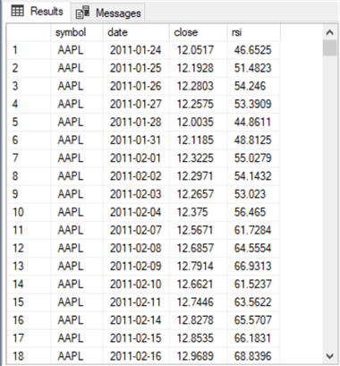
The following screen shot is for the first 18 rows in the rsi_and_close_values table. As you can see these are for the first eighteen trading dates in 2011 with both close and rsi column values for the AAPL ticker.

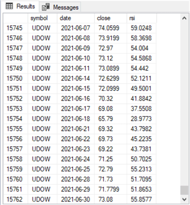
The next screen shot is for the last 18 rows in the rsi_and_close_values table. As you can see these are for the last eighteen trading dates ending on June 30 in 2021 with both close and rsi column values for the UDOW ticker.

One model with two parameter sets

You can simulate strategies for trading based on historical RSI values and close prices with T-SQL code. This section presents and describes T-SQL code for evaluating two variations of an RSI security trading strategy. By simulating two or more variations, you can compare the results to assess which strategy variation yields the more profitable outcomes for a set of securities over a timeframe.

A common strategy for buying and selling securities is to buy a security when its RSI value rises from below 30 to above 30 and then then sell the security when its RSI value falls from above 70 to below 70.
Another variation of the preceding strategy is to buy a security when its RSI value rises from below 40 to above 40 and then sell the security when its RSI value falls from above 70 to below 70.

This section presents and describes the T-SQL code for implementing these two strategies. The results for each strategy is computed for the six ticker symbols in the rsi_and_close_values table that are populated in the preceding section. Buy-sell cycles are created for each ticker symbol over the nine and a half years of computed RSI values. The close values in the rsi_and_close_values table reflect the price at which securities are bought and sold, respectively, for buy and sell signals.

The rest of this section walks through the code for implementing the first of the two strategies. This tip's download includes two T-SQL scripts – one for each trading strategy mentioned above.

The code starts with the setup for a while loop that is similar to the code in the preceding section for populating the rsi_and_close_values table. Then, in the body of the while loop, the following processing steps are implemented.

The excerpt below starts by deleting any prior version of the #for_buy_sell_30_70 temp table.
Next, the script excerpt populates the temp table based on the rsi_and_close_values table from the into clause of a select statement. The select statement also adds two new columns. The columns named from_lt_30_to_gt_30 and from_gt_70_to_lt_70, respectively, mark candidate rows for buying and selling a security.

drop table if exists #for_buy_sell_30_70
 
select 
 rsi_and_close_values.symbol
,rsi_and_close_values.date
,rsi_and_close_values.[close] [close]
,rsi current_rsi
,
 case
  when rsi > 30
   and lag(rsi_and_close_values.rsi, 1) over (order by rsi_and_close_values.date) < 30
  then 'buy signal'
 end from_lt_30_to_gt_30
,
 case
  when rsi < 70
   and lag(rsi_and_close_values.rsi, 1) over (order by rsi_and_close_values.date) > 70
  then 'sell signal'
 end from_gt_70_to_lt_70
into #for_buy_sell_30_70
from dbo.rsi_and_close_values
where rsi_and_close_values.symbol = @symbol  
order by rsi_and_close_values.symbol,rsi_and_close_values.date

Here are a couple of excerpts from the results set in the #for_buy_sell_30_70 temp table.

The first excerpt shows the first twenty-one days for rsi values. There are a couple of sell signal rows in this timeframe, but no buy signal rows.
The second excerpt shows the first pair of rows with buy signals.
- These two buy signal rows are separated by just one trading date.
- Furthermore, there is no sell signal row between the first and second buy signal rows.
The data in the #for_buy_sell_30_70 temp table clearly requires further processing to identify the first and last dates for each buy-sell cycle in a succession of buy-sell cycles.

The next code excerpt is a nested query that extracts just those buy signal rows that are preceded by a sell signal row.

The inner-most query named for_first_buy_signal returns all rows for a symbol that have the string “buy signal” in the from_lt_30_to_gt_30 column or the string “sell signal” in the from_gt_70_to_lt_70 column.
The outer-most query further restricts the query's results set to just those rows with a buy_signal column value of “buy signal” and a preceding row (from_prior_sell_signal) with a “sell signal” column value.

-- list first buy signal rows
drop table if exists #first_buy_signal_30_rows
 
-- first buy signal row code
-- look for buy signal rows right after prior sell signal rows
select *
into #first_buy_signal_30_rows
from
(
select 
 symbol
,date
,[close] [close]
,current_rsi
,from_lt_30_to_gt_30 buy_signal
,from_gt_70_to_lt_70 sell_signal
,lag(from_gt_70_to_lt_70,1) over (order by date) from_prior_sell_signal
from #for_buy_sell_30_70
where from_lt_30_to_gt_30 = 'buy signal'
 or from_gt_70_to_lt_70 = 'sell signal'
) for_first_buy_signal
where buy_signal = 'buy signal'
and from_prior_sell_signal = 'sell signal'

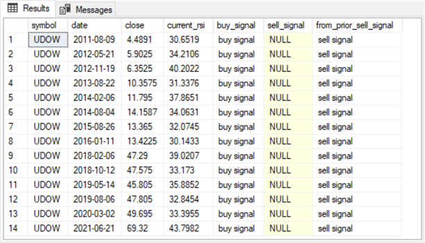
The following screen shot shows the results set from the #first_buy_signal_30_rows temp table populated by the preceding script.

There are fourteen rows in the results set.
The first row corresponds to the first row in the preceding screen shot for unfiltered buy signal rows.

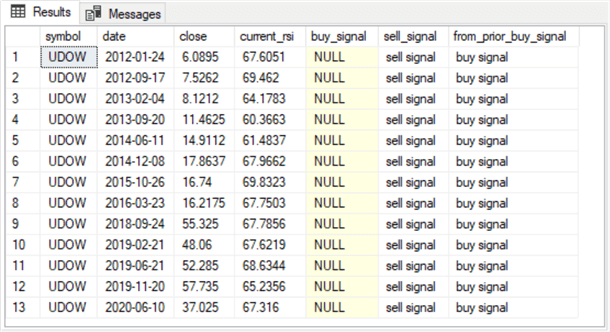
The next code excerpt is for sell signal rows that are preceded by a buy signal. The screen shot below the code excerpt is for the results set stored in the #first_sell_signal_70_rows temp table. Notice there are just thirteen rows in this results set. The preceding results set from the #first_buy_signal_30_rows temp table had fourteen rows. The extra row in the #first_buy_signal_30_rows results set is present because the underlying data starts a buy signal for a buy-sell cycle after the thirteenth sell signal, but the timeframe for computing RSI values ends before the matching sell signal row. Therefore, the fourteenth row in the preceding screen is an orphaned buy signal because it has no matching sell signal row to end the buy-sell cycle that it starts.

-- list first sell signal rows
drop table if exists #first_sell_signal_70_rows
 
-- first sell signal
-- look for sell signal rows right after prior buy signal rows 
select *
into #first_sell_signal_70_rows
from
(
select 
 symbol
,date
,[close] [close]
,current_rsi
,from_lt_30_to_gt_30 buy_signal
,from_gt_70_to_lt_70 sell_signal
,lag(from_lt_30_to_gt_30,1) over (order by date) from_prior_buy_signal
from #for_buy_sell_30_70
where from_lt_30_to_gt_30 = 'buy signal'
 or from_gt_70_to_lt_70 = 'sell signal'
) for_first_buy_signal
where sell_signal = 'sell signal'
and from_prior_buy_signal = 'buy signal'

The last processing step to complete the code for implementing the first trading strategy based on RSI values has two main goals. First, it concatenates the results sets from the #first_buy_signal_30_rows and #first_sell_signal_70_rows tables. Second, it removes any buy signal rows without a matching sell signal rows that trails it. The second step also removes from the final results set in the #buy_sell_30_70_cycles temp table any sell signal row that starts a buy-sell cycle results set. This is because a buy-sell cycle can only start with a buy signal. Here's the code for the last processing step.

-- concatenate #first_buy_signal_30_rows 
-- and #first_sell_signal_70_rows
-- into buy_sell_30_70_cycles
 
drop table if exists #buy_sell_30_70_cycles
 
select 
 symbol
,[date] date
,[close] [close]
,current_rsi
,buy_signal
,sell_signal
into #buy_sell_30_70_cycles
from
(
select * from #first_buy_signal_30_rows
union
select * from #first_sell_signal_70_rows
) for_#buy_sell_30_70_cycles
order by date
 
-- select * from #buy_sell_30_70_cycles
 
 
-- drop first row in #buy_sell_30_70_cycles if sell_signal column value equals 'sell signal'
-- to remove an initial sell signal
if (select top 1 sell_signal from #buy_sell_30_70_cycles) = 'sell signal'
   delete from #buy_sell_30_70_cycles where date = (select min(date) from #buy_sell_30_70_cycles)
 
-- drop last row in #buy_sell_30_70_cycles if row count is odd
-- to remove a trailing buy signal
if (select (select count(*) num from #buy_sell_30_70_cycles) % 2) = 1
   delete from #buy_sell_30_70_cycles where date = (select max(date) from #buy_sell_30_70_cycles)
 
-- display #buy_sell_30_70_cycles
select * from #buy_sell_30_70_cycles

Here's the results set from in the final processing step for the first set of parameters used with the RSI model examined in this tip. Notice there are just twenty-six rows in this results set. The union operator in the preceding code excerpt concatenates the results sets for buy signal rows and sell signal rows. The second if statement and its trailing delete statement removes the last buy signal row, which has no matching sell signal row.

The T-SQL code for simulating trading based on the second set of parameters is nearly the same as for the first set of parameters. The main differences in the code for the second set of parameters are for the first code block where rows are pulled from the rsi_and_close_values table into a new table whose derivations are successively reprocessed to finally arrive at new table with the buy-sell rows.

The parameters for second set of parameters specify the buying of a security when the RSI value for a trading date rises from below 40 to above 40.
The first set of parameters specify, in contrast, the buying of a security only when the RSI value for a trading date rises from below 30 to above 30.
Both the first and second parameter sets have the same rule for selling a security. Sell the security when RSI value declines from above 70 to below 70.

Here is the code excerpt showing the initial query for the second parameter set.

The name of the table that it creates and populates is #for_buy_sell_40_70 instead of #for_buy_sell_30_70.
An even more critical difference for the code that designates buy and sell actions is the specification of a new case statement for the column on which buy decisions are made.
- The name of the new column for the second parameter set is from_lt_40_to_gt_40. This name signifies that buy decisions are made when the RSI value rises from below 40 to above 40.
- The comparable column in the code for the first parameter set has the name from_lt_30_to_gt_30.

drop table if exists #for_buy_sell_40_70
 
select 
 rsi_and_close_values.symbol
,rsi_and_close_values.date
,rsi_and_close_values.[close] [close]
,rsi current_rsi
,
 case
  when rsi > 40
   and lag(rsi_and_close_values.rsi, 1) over (order by rsi_and_close_values.date) < 40
  then 'buy signal'
 end from_lt_40_to_gt_40
,
 case
  when rsi < 70
   and lag(rsi_and_close_values.rsi, 1) over (order by rsi_and_close_values.date) > 70
  then 'sell signal'
 end from_gt_70_to_lt_70
into #for_buy_sell_40_70
from dbo.rsi_and_close_values
where rsi_and_close_values.symbol = @symbol
order by rsi_and_close_values.symbol,rsi_and_close_values.date

Perhaps the best way to appreciate the differences in the code for processing the rsi_and_close_values table from the second parameter set versus first parameter set is to examine the final results set of buy-sell rows from the second parameter set versus first parameter set. The next screen shot shows the final buy-sell results set from the second parameter set. It can be compared to the preceding screen shot showing the comparable results set from the first parameter set.

One especially obvious difference is that there are 18 buy-sell pairs with a total of 36 rows for the second parameter set, but there are only 13 buy-sell pairs with a total of 26 rows for the first parameter set. Therefore, the second parameter set allows ten more tries to accumulate gains relative to the first parameter set.
In addition to the number of buy-sell dates being different for the two parameter sets, the dates for the buy-sell pairs are typically different as well.
- The initial buy date for the second parameter set is on 2011-03-18 whereas the initial buy date for the first parameter set is much later (2011-08-09).
- The final sell date for the second parameter set is 2021-02-25 versus a final sell date of 2020-06-10 for the first parameter set.
- As you can see, the second parameter set starts making buy decisions before the first parameter set, and the second parameter set also continues making sell decisions after the first parameter set stops making sell decisions.

Comparing Growth Rates Between model parameter sets

At this point in the tip, it is reasonable to ask: which set of parameters yield the best results? There is no easy answer to the question because the answer can depend on which securities you are tracking and for what timeframe you are tracking them. However, it is relatively easy to answer the question of what is the compound annual growth rate (CAGR) of the securities tracked in this tip for the nine and a half years for which this tip reports results. The CAGR is the average annual rate of returns from an investment starting at a beginning balance and running through an ending balance assuming the gains (or losses) are applied to the balance at end of each trade through the end of trading.

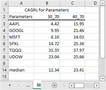
Here is a summary table of the CAGR values across security tickers tracked in this tip for each of the two parameter sets. The six tickers go down the side, and two parameter sets are referenced in column headers.

As you can see, the parameter set that buys when the RSI value crosses from below to above a value of 40 does consistently better across the six tickers in this tip than the parameter set that crosses from below to above a value of 30.
The median CAGR across tickers is 12.34 for the 30 and 70 parameter set, but median CAGR jumps to about twice that amount for the 40 and 70 parameter set.
The 40 and 70 parameter set consistently generates superior returns than the 30 and 70 parameter set, but there is also a substantial tendency for results to vary by ticker symbol.
- For example, the AAPL ticker has a CAGR OF 4.42 with the 30 and 70 parameter set.
- However, the TQQQ ticker with the 30 and 70 ticker set has a CAGR of 33.35.

There are 13 pairs of buy-sell pairs for the TQQQ ticker with 30 and 70 parameter set.

The following excerpt from an Excel worksheet tab shows the buy-sell pairs in columns A through G copied from the Results tab of a SSMS Results tab.
Columns I and J contain entered and computed values in the worksheet
- Cell J1 is a beginning account balance of $1000 for the TQQQ ticker. This is an entered value.
- The buy and sell dates for the first buy-sell cycle are 3/17/2011 and 5/2/2011, respectively.
- The percentage gain in account balance at the end of the first buy-sell cycle is about 26% (examine cell I3). This is a computed value.
- At the end of the first buy-sell cycle the balance grew to $1,256.46 (view cell J3).
- Just before the last buy-sell cycle, the TQQQ account balance grew to $16.236.83. This value appears in cell J25.
- During the last buy-sell cycle, the TQQQ account balance declined by around 5 percent to an ending balance of $15,400.04 (see cell J27).
- The value just below the cell with num of years is the inverse of 9.5 – namely, about .105263158; there are 9.5 years from the start of 2011 through the June 20, 2021, which is the last possible ending date in this tip. This is the second entered value in columns I and J. The other populated cells in columns I and J contain computed values by expressions within the worksheet.
- The equation for the compound aggregate growth rate (cagr) is as follows

(((EndingBalance/BeginningBalance)^InverseOfNumberOfYears)-1)*100

The computed cagr value appears in cell I32; this value matches the one that appears in cell B7 of the preceding screen shot.

Next Steps

The main purpose of this tip is to introduce you to T-SQL coding techniques for choosing a buy date and a sell date based on RSI values. One simple model was specified, coded, and interpreted for two different parameter sets. The parameter set that bought a security when its RSI value crosses from below 40 to above 40 yielded more profitable returns than the parameter set that bought a security when its RSI value crosses from below 30 to above 30.

There are three files in the download for this tip.

The first file contains csv formatted values with open, high, load, close and volume values for the six tickers in this tip over the timeframe from the beginning of January in 2011 through June 30 in 2021. To run the sample code you will need to transfer this csv file to a SQL Server table (for example, one named yahoo_finance_ohlcv_values_with_symbol in the dbo schema of the DataScience database).
The next file contains a sql script block with three main T-SQL code segments.
- One segment is for computing RSI values from the csv data after its values are copied to a SQL Serve table.
- The other two segments are sql scripts for generating buy-sell pairs based on each of the two parameter sets. The scripts for each parameter sets generates results for each of the six tickers in the tip.
The final file is an Excel workbook file with the results reported in this tip's third section.

The obvious next step is to load the source csv data into a SQL Server table and then run the sql script files to obtain the outcomes reported in this tip. Another next step would be to compare the outcomes for the buy-sell pairs in this tip to other tips reporting results for different models (for example, compare the results in the current tip to those in this prior tip).

About the author

Rick Dobson is an author and an individual trader. He is also a SQL Server professional with decades of T-SQL experience that includes authoring books, running a national seminar practice, working for businesses on finance and healthcare development projects, and serving as a regular contributor to MSSQLTips.com. He has been growing his Python skills for more than the past half decade -- especially for data visualization and ETL tasks with JSON and CSV files. His most recent professional passions include financial time series data and analyses, AI models, and statistics. He believes the proper application of these skills can help traders and investors to make more profitable decisions.

This author pledges the content of this article is based on professional experience and not AI generated.

View all my tips

Article Last Updated: 2022-06-17

Using T-SQL and the RSI to Predict When to Buy and Sell Financial Securities