Revisiting Time Series Model Performance Assessment with T-SQL

By: Rick Dobson   |   Updated: 2022-04-27   |   Comments   |   Related: > TSQL

Problem

As a SQL Server professional and an aspiring data scientist, I am interested in learning about ways to build models for time series data and assess the performance of those models. More specifically, I want to assess model performance for different ticker symbols and/or the same tickers over different time periods. Please present a SQL-based demonstration that shows how to implement these kinds of assessments as well as a framework for projecting results to a larger domain of tickers than those used in assessing model performance.

Solution

Three prior tips introduce T-SQL developers to techniques for formulating, implementing and assessing time series models based on exponential moving average crossovers. A crossover is when a moving average of one period length crosses above or below an exponential moving average with another period length. Crossovers are frequently associated with trend reversals, such as from trending down to trending up and vice versa.

• The first tip titled "Model and Log Trend Reversals for Time Series Data in SQL Server" shows how to use T-SQL in SQL Server to model trend reversals in time series data.
• The second tip titled "Create and Compare SQL Time Series Models" reveals a rudimentary framework for comparing two or more models.
• The third tip titled "Assessing Time Series Model Performance with T-SQL" illustrates a couple of statistics for assessing which of two models perform better.

This tip focuses on models that specify when to buy and sell a financial security with the objective of growing an account balance through successive trades over time. With a sufficient amount of creativity, a data scientist and a SQL Server professional can adapt the approach to other contexts. The Engineering and Statistics Handbook lists these use cases for time series analysis: economic forecasting, sales forecasting, process and quality control, inventory studies, and census analysis.

This tip builds on the three prior tips in the following ways.

• First, the sample data in this tip is composed to be representative at a sector level to the overall US stock market. The sample for the prior three tips referenced at the top of this section is based on ticker symbols that I was following at the time that I authored the tips.
• Second, nearly twice as many ticker symbols and more than twice the amount of historical data per ticker symbol are examined in this tip relative to the three prior tips. This tip's enhanced sample enriches the proper interpretation of model performance outcomes.
• Third, two statistics for assessing model performance are coded in T-SQL so there is no need to copy data from SQL Server to Excel to compute performance metrics. This enhances the automation of an assessment framework.
• Finally, this tip concludes with an integrated analysis of time series explicitly selected for the current tip as well as the time series from the third tip referenced at the top of this section.

This tip assumes a basic level of familiarity with exponential moving averages. If you are not familiar with exponential moving averages, you can refer to this prior tip which includes a general explanation of exponential moving averages and period lengths. The prior tip also includes T-SQL code samples for computing ten-period and twenty-period exponential moving averages.

T-SQL for a pair of time series models

This tip drills down on the assessment of two T-SQL models for time series data. Both models look for reversals in a pair of exponential moving averages having different period lengths.

• The first model searches for a succession of adjacent stock trading days when a ten-period length exponential moving average (ema_10) crosses from below in the prior period to above in the current period for an exponential moving average with a period length of twenty periods (ema_20). The first model also searches for the reverse relationship of the exponential moving averages in adjacent time periods.
  • When ema_10 is above ema_20 in the current period and ema_10 is less than or equal to ema_20 in the prior period, then the first model posts a buy signal in the buy_sell_signal column of its log. This is because prices are moving up across the two adjacent time periods.
  • When ema_20 is greater than ema_10 in the current period and ema_10 is greater than or equal to ema_20 in the prior period, then the first model posts a sell signal in the buy_sell_signal column of its log. This is because prices are moving down across the two adjacent time periods.
  • When there is no cross-over between ema_10 and ema_20 from the prior to the current trading day, the buy_sell_signal column in the model's log is left NULL. This is because prices are not reversing from trending either up or down across the two periods.
• The second model uses a different pair of exponential moving averages for determining when to post buy signal and sell signal values in the buy_sell_signal column in the model's log.
  • When ema_10 is greater than ema_20 in the current period and ema_30 is less than or equal to ema_10 in the prior period, then the second model posts a buy signal in the buy_sell_signal column of its log.
  • When ema_20 is greater than ema_10 in the current period and ema_10 is greater than or equal to ema_30 in the prior period, then the second model posts a sell signal in the buy_sell_signal column of its log.
• Notice that the first model uses the same exponential moving averages (ema_10 and ema_20) in the criteria for the current and the prior periods. Using the same criteria with a reversed relationship for buy and sell signals causes the two signal types to switch from one type to the other in a sequential order. That is, each buy signal is followed by a sell signal and vice versa.
• However, the buy and the sell signals in the log for the second model do not necessarily follow each other in the same precise way as in the first model.
  • For example, there can be multiple buy signals following the first buy signal in a buy-sell cycle.
  • Likewise, there can be multiple sell signals after the first sell signal in a buy-sell cycle before the next buy signal for a new buy-sell cycle.
  • It is possible to ignore the repeat buy signals in a buy-sell cycle and the repeat sell signals between the sell signal in one buy-sell cycle and the buy signal for the next buy-sell cycle.
  • Custom code for both the first and second models ignores "repeat" buy and sell signals. This code is described in detail in the "T-SQL code for deriving buy-sell cycle dates for a symbol from a log table" section of an earlier tip.
  • There is one more special feature for the code implementing the first and second models. Earlier versions of the code for the models relied on an external processing to make sure that the log for each model started with a buy signal and ended with a sell signal. This external step was necessary because a buy-sell cycle must start on the period after a buy signal and end on the period after a sell signal. An updated version of the code within this tip has a new feature to automatically enforce this rule without the need for any external filtering of the model logs.

Here are excerpts from the code for the first model for the eleven ticker symbols used in this tip. The main objective of the code excerpts is to illustrate key elements for populating a log table (symbol_temp_log) for the first ticker symbol (AMT) based on the contents of the log_for_buy_at_ema_10_gt_20 table, which contains data for all eleven tickers. Complete scripts for both the first model and the second model appear in this tip's download.

• The script excerpt below starts with a SSMS use statement to specify a default database. The database name is DataScience, but you can reference any database with the time series data for the model you are assessing. If you use a different database name than DataScience, you may have to update selected references to DataScience in the scripts for the first and second models.
• The first code block after the use statement populates the log_for_buy_at_ema_10_gt_20 table. This table is populated from a subquery named for_buy_sell_log_for_ema_10_vs_20. The subquery code does not show below to keep the focus on the model logic and key elements for implementing the model with T-SQL.
• The subquery named for_buy_sell_log_for_ema_10_vs_20 returns raw time series data, computed exponential moving averages, and selected other computed fields required by the model.
• The outer query referencing the subquery assigns buy signal or sell signal values to selected rows in the buy_sell_signal column in the log_for_buy_at_ema_10_gt_20 table.
• The outer query also assigns open price values to the buy_sell_price column in the log_for_buy_at_ema_10_gt_20 table.
• The decision about which rows to write buy signal and sell signal values along with corresponding open price values is determined by a pair of case statements with when clauses based on exponential moving average value comparisons.
• The outer query in the script excerpt below is trailed by a pair of double—dashed comment marker lines that divide the first code block from the second code block.

The second code block starts immediately after the pair of double—dashed comment marker lines.

• The main objective of the second code block is to extract rows for a specific ticker symbol (AMT) and to populate a new fresh version of a log table which is for just one ticker symbol instead of all eleven ticker symbols.
  • The new log table is saved in the symbol_temp_log table via the into clause for a select statement
  • The @symbol local variable is assigned the ticker symbol value for one of the eleven distinct ticker symbols in the log_for_buy_at_ema_10_gt_20 table.
• Another objective of the second code block is to declare local variables with names of @first_buy_signal_date through @next_sell_signal_date. These local variables are used in subsequent code that cleans up cases where there are repeat buy signal values in a buy-sell cycle and/or repeat sell signal values between buy-sell cycles. This subsequent code does not appear in the tip, but it is included in the tip's download.
• A third objective of the second code block is to assign NULL values to selected columns for any sell signal row that starts the log for a symbol or any buy signal row that ends the log for a symbol. Recall that buy-sell cycles require both a buy signal and a sell signal.

use DataScience
go
 
-- create the log for all symbols
drop table if exists dbo.log_for_buy_at_ema_10_gt_20
 
-- create dbo.log_for_buy_at_ema_10_gt_20
select 
 date
,symbol
,[open]
,[close]
,ema_10_lag_1
,ema_20_lag_1
,ema_10
,ema_20
 
-- set buy and sell signals
,case
   when ((ema_10_lag_1 <= ema_20_lag_1) and (ema_10 > ema_20)) then 'buy signal'
   when ((ema_10_lag_1 >= ema_20_lag_1) and (ema_20 > ema_10)) then 'sell signal'
   else null
 end buy_sell_signal
 
-- set buy and sell prices
,case
   when ((ema_10_lag_1 <= ema_20_lag_1) and  (ema_10 > ema_20)) then open_lead_1
   when ((ema_10_lag_1 >= ema_20_lag_1) and (ema_20 > ema_10)) then open_lead_1
   else null
 end buy_sell_price
 
into dbo.log_for_buy_at_ema_10_gt_20
 
from
(
-- source time series data rows for buy/sell actions
-- see the download for the code in the subquery
) for_buy_sell_log_for_ema_10_vs_20
 
 
-- optionally display the log for all symbols for all dates
-- select * from dbo.log_for_buy_at_ema_10_gt_20
go
 
--------------------------------------------------------------------------------------
--------------------------------------------------------------------------------------
 
-- Prepare for cleaning the log for AMT
 
-- declarations
declare 
    @symbol nvarchar(10) = 'AMT'
   ,@first_buy_signal_date date
   ,@first_sell_signal_date date
   ,@prior_buy_signal_date date
   ,@prior_sell_signal_date date
   ,@next_buy_signal_date date
   ,@next_sell_signal_date date
 
-- create and populate a temp log for a symbol 
-- with buy_sell_signal dates (next_date)
drop table if exists dbo.symbol_temp_log
 
select [date]
      ,[symbol]
      ,[open]
      ,[close]
      ,[ema_10_lag_1]
      ,[ema_20_lag_1]
      ,[ema_10]
      ,[ema_20]
      ,[buy_sell_signal]
      ,[buy_sell_price]
      ,lead(date,1) over (partition by symbol order by date) next_date
into dbo.symbol_temp_log
from dbo.log_for_buy_at_ema_10_gt_20
where symbol = @symbol
 
-- NULL buy_sell_signal and buy_sell_price
-- if first sell signal is before first buy signal
if (select min(next_date)
from symbol_temp_log
where buy_sell_signal = 'sell signal')
<
(select min(next_date) 
from symbol_temp_log
where buy_sell_signal = 'buy signal')
 
   update symbol_temp_log
   set buy_sell_signal = NULL, buy_sell_price = NULL
   where next_date = (select min(next_date)
   from symbol_temp_log
   where buy_sell_signal = 'sell signal')
 
-- NULL buy_sell_signal and buy_sell_price
-- if last buy signal is after last sell signal
if (select max(next_date)
from symbol_temp_log
where buy_sell_signal = 'buy signal')
>
(select max(next_date) 
from symbol_temp_log
where buy_sell_signal = 'sell signal')
 
   update symbol_temp_log
   set buy_sell_signal = NULL, buy_sell_price = NULL
   where next_date = (select max(next_date)
   from symbol_temp_log
   where buy_sell_signal = 'buy signal')
 
-- optionally echo two resource tables
-- log for all symbols
-- select * from dbo.log_for_buy_at_ema_10_gt_20
-- log for current symbol
select * from dbo.symbol_temp_log

Here are comparable excerpts for the second model. There is one key distinction between the code for the first and second models.

• Recall that the first code segment populates the log_for_buy_at_ema_10_gt_20 table with the log for all eleven ticker symbols used in this tip. This table is freshly populated for the second model.
• Notice that the first code segment references different exponential moving averages for the prior period in its case statements.
  • The code for the second model below compares ema_30 to ema_10 in its prior period,
  • but the code for the first model above compares ema_20 to ema_10.
• The first and second models compare the same exponential moving averages for the current period – namely, ema_20 and ema_10.
• As a result, the second model requires the exponential moving value in the prior period to be farther below the ema_10 value in the prior period. However, the second model requires the current period to rise to the same level as the first model.
• Therefore, the second model references a deeper trend reversal that does the first model.

Use DataScience
go
 
-- create the log for all symbols
drop table if exists dbo.log_for_buy_at_ema_10_gt_20
 
-- create dbo.log_for_buy_at_ema_10_gt_20
select 
 date
,symbol
,[open]
,[close]
,ema_10_lag_1
,ema_30_lag_1
,ema_10
,ema_20
 
-- set buy and sell signals
,case
   when ((ema_10_lag_1 <= ema_30_lag_1) and (ema_10 > ema_20)) then 'buy signal'
   when ((ema_10_lag_1 >= ema_30_lag_1) and (ema_20 > ema_10)) then 'sell signal'
   else null
 end buy_sell_signal
 
-- set buy and sell prices
,case
   when ((ema_10_lag_1 <= ema_30_lag_1) and(ema_10 > ema_20)) then open_lead_1
   when ((ema_10_lag_1 >= ema_30_lag_1) and (ema_20 > ema_10)) then open_lead_1
   else null
 end buy_sell_price
 
into dbo.log_for_buy_at_ema_10_gt_20
 
from
(
-- source rows for buy/sell actions
select 
-- source time series data rows for buy/sell actions
-- see the download for the code in the subquery
) for_buy_sell_log_for_ema_10_vs_20
 
go
 
--------------------------------------------------------------------------------------
--------------------------------------------------------------------------------------
--/*
 
-- Prepare for cleaning the log for AMT
 
-- declarations
declare 
   @symbol nvarchar(10) = 'AMT'
   ,@first_buy_signal_date date
   ,@first_sell_signal_date date
   ,@prior_buy_signal_date date
   ,@prior_sell_signal_date date
   ,@next_buy_signal_date date
   ,@next_sell_signal_date date
 
-- create and populate a temp log for a symbol 
-- with buy_sell_signal dates (next_date)
drop table if exists dbo.symbol_temp_log
 
select [date]
      ,[symbol]
      ,[open]
      ,[close]
      ,[ema_10_lag_1]
      ,[ema_30_lag_1]
      ,[ema_10]
      ,[ema_20]
      ,[buy_sell_signal]
      ,[buy_sell_price]
     ,lead(date,1) over (partition by symbol order by date) next_date
into dbo.symbol_temp_log
from [dbo].[log_for_buy_at_ema_10_gt_20]
where symbol = @symbol
 
-- NULL buy_sell_signal and buy_sell_price
-- if first sell signal is before first buy signal
if (select min(next_date)
from symbol_temp_log
where buy_sell_signal = 'sell signal')
<
(select min(next_date) 
from symbol_temp_log
where buy_sell_signal = 'buy signal')
 
   update symbol_temp_log
   set buy_sell_signal = NULL, buy_sell_price = NULL
   where next_date = (select min(next_date)
   from symbol_temp_log
   where buy_sell_signal = 'sell signal')
 
-- NULL buy_sell_signal and buy_sell_price
-- if last buy signal is after last sell signal
if (select max(next_date)
from symbol_temp_log
where buy_sell_signal = 'buy signal')
>
(select max(next_date) 
from symbol_temp_log
where buy_sell_signal = 'sell signal')
 
   update symbol_temp_log
   set buy_sell_signal = NULL, buy_sell_price = NULL
   where next_date = (select max(next_date)
   from symbol_temp_log
   where buy_sell_signal = 'buy signal')
 
-- optionally echo two resource tables
-- log for all symbols
-- select * from dbo.log_for_buy_at_ema_10_gt_20
-- log for current symbol
select * from dbo.symbol_temp_log

Review of results sets from two models

The preceding section shows and discusses excerpts from the T-SQL code for the first model and the second model.

• The excerpts show the first part of how to create the log for a single ticker symbol. The model's log is the first results set from the code for each model.
• The second results set is derived by reading and processing the log from a model.
  • The processing extracts from the log for each model pairs of buy and sell dates and prices. A buy date with its matching sell date comprises a buy-sell cycle. The price change – either positive or negative -- during a buy-sell cycle can update the prior current balance associated with a model. These changes in the current balance reveal the performance of each model for altering an initial account balance over a sequence of buy and sell dates for a ticker symbol.
  • The log results set as well as the results set of buy and sell dates and prices are for a set of ticker symbols. There are eleven tickers in this tip – one for each of the Standard and Poor's sectors. The ticker symbols by sector are
    • AMT for Real Estate
    • AMZN for Consumer Cyclical
    • HON for Industrials
    • JNJ for Healthcare
    • JPM for Financial
    • MSFT for Technology
    • NEE for Utilities
    • PG for Consumer Defensive
    • SHW for Materials
    • VZ for Communications Services
    • XOM for Energy
• The third results set is for tracking the performance of a model for changing an initial account balance into an ending account balance. This tip tracks model performance with two metrics, but special attention is paid to one metric.
  • The Rate of Change metric tracks the percentage change of the account balance from before the first buy-sell cycle through the final buy-sell cycle for a model. For this tip, the evaluation period is from the beginning of January 2000 through February 18, 2022.
  • The Compound Annual Growth Rate (CAGR) tracks the average annual change in value for an investment from an initial account balance through a final account balance over a timeframe in years. In the context of this tip, the evaluation duration is approximately 22.13 years. This metric only requires the beginning balance and the ending balance as well as the evaluation timeframe.
  • The initial balance for both models for each ticker symbol is $1,000. The ending balance is computed in by a model's script. The ending balance depends on the model's design and its interaction with the time series data for a ticker symbol.

The following screen shot shows a Results tab view with contents excerpted from the first model's results sets. These outcomes are for the AMT ticker symbol.

• The first window in the Results tab is for the first results set. This window shows rows from the beginning of the model's log. There is a separate row for each trading date.
• As you can see, the row for January 6, 2000 is selected. This date is for the buying of a security. The buy signal is on the preceding row (the one for January 5, 2000) because the model bases its decision about when to buy based on exponential moving averages for close values which are not known until after the close of a trading day. The buy is executed at the open price of the next trading date. Therefore, the buy price is the open price (29.4375) on January 6.
• The second window for a ticker symbol shows the buy-sell cycle dates and prices along with selected other values. Each buy-sell cycle is represented by a pair of two successive rows. The first row in a pair is for the buy in a buy-sell cycle, and the second row in a sample is for the sell in a buy-sell cycle.
  • For example, the highlighted row is for a buy for the log entry selected in the top window. The buy for the first buy-sell cycle corresponds to a buy signal in the row with a date column value of January 5, 2000; this is the trading date before the actual buy action on January 6, 2000.
  • The first sell from the first model for AMT appears in the second row in the second results set. This row's buy_sell_cycle_date column value is April 5, 2000, which corresponds to a sell signal issued after the close of trading on April 4, 2000.
  • The percentage price change is the sell price less the buy price (44.00 – 29.4375) divided by the buy price – namely, 49.46 percentage points.
  • The current balance at the end of the first buy-sell cycle is percentage price change during the first buy-sell cycle times the initial current balance, which is $1,000 before the first buy-sell cycle.
• The third window in the following screen shot displays assessment results.
  • The first model's ending current balance is 6790.12. This is the cumulative current balance across all the buy-sell cycles.
  • The Rate of Change is the ending current balance (6790.12) less the initial current balance (1000) divided by the initial current balance less 1 times 100, which equals 579.01 percent.
  • The compound annual growth rate (CAGR) is based on the ending current balance divided by the initial current balance raised to the inverse of the timeframe for which a model is being evaluated; this raised value is reduced by 1. For this tip, the timeframe is 22.13 years, and the inverse of this in years is (1/22.13). Because the results of the CAGR expression is a percentage, it is multiplied by 100 to make it comparable to the Rate of Change percentage. The CAGR percentage value is 9.04 percent. This means
  • the initial current balance grows to the ending current balance at a compound rate of 9.04 percent for each of the 22.13 years during which the model is evaluated.

The following screen shot shows a Results tab view with contents excerpted from the second model's results sets. These outcomes are also for the AMT ticker symbol. Just as there is a separate set of three results sets for the first and second models, there are also separate sets of the results sets for each of the remaining ten tickers examined in this tip.

• If you carefully examine the second window from the preceding and the following screen shot, you will notice that they have identical current values at the end of the first buy-sell cycle. This is because the first and second models derive the same buy and sell dates for the first buy-sell cycle. This is a result of their model parameters.
• On the other hand, the current values at the end of subsequent buy-sell models diverge between the two models. This reflects the model parameters for the first and second models.
• As a result of the divergence in model performance over the buy-sell cycles specified by each model, the assessments of model performance are different for different models. For example, the CAGR value is 5.48 for the second model, but the preceding screen shot shows the CAGR value is 9.04 for the first model. This means that the first model delivers superior performance to the second model for the AMT ticker.

Assessing time series model performance

This section presents and describes CAGR comparative values for three sets of data

• The 11 ticker symbols examined in this tip; all the data from this tip is for an evaluation range from January 2000 through February 18, 2022.
• The 6 ticker symbols examined in a prior model assessment tip; all the data from the prior tip is for an evaluation range from January 2011 through June 30, 2021.
• A combined set of time series with the 11 tickers for the time series in this tip and 6 tickers with the time series from the prior tip. There is one ticker (MSFT) that is in both sets of time series data, but the evaluation dates are different – namely, January 2000 through February 18, 2022 for the current tip and January 2011 through June 30, 2021 for the prior tip.

The purposes for performing the comparisons are

• To reveal which model generates the most positive CAGR values across the ticker symbols
• To determine if model 1 outcomes can predict model 2 outcomes and to show the outcomes from each model
• To illustrate whether it is possible to combine the outcomes from the two models and obtain a consistent result

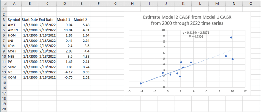
Here is an excerpt from a tab from an Excel workbook that compares the first model (Model 1) and the second model (Model 2) examined in this tip.

• Column A shows each of the eleven ticker symbols.
• Column D shows the CAGR values from Model 1. These values were derived from the assessment window for each ticker symbol.
• Column E shows the CAGR values from Model 2. These values were also derived from the assessment window for each ticker symbol.
• For 8 of 11 tickers, the Model 2 CAGR value are greater than the Model 1 CAGR value.
• The chart to the right within the spreadsheet below shows a linear regression for the prediction of Model 2 CAGR values from Model 1 CAGR values. The R² value for the linear regression is statistically different from 0 at beyond the .05 level. This outcome confirms a linear relationship between Model 2 CAGR values and Model 1 CAGR values. As the Model 1 CAGR for a ticker grows so does the Model 2 CAGR value.

Here is an excerpt from a tab from an Excel workbook that compares the first model (Model 1) and the second model (Model 2) examined in the prior tip.

• The tickers, with one exception for MSFT, are different in the prior tip from those in this tip.
  • The tickers in this tip are selected so that there is one large cap ticker symbol for each of the 11 major ticker sectors.
  • The tickers in the prior tip are of two types.
    • Three of the six tickers (AAPL, GOOGL, and MSFT) are from the Technology sector.
    • The other three tickers are triple levered exchange traded funds based on the DOW, S&P 500, and NASDAQ composite indexes (UDOW, SPXL, and NASDAQ).
  • The data from this tip and the prior tip are also different in the timeframe used to evaluate CAGR values. The different date ranges are specified at the beginning of this section.
• With one exception (AAPL), The Model 2 CAGR values are greater than the corresponding Model 1 CAGR values.
• A linear relationship between the Model 1 CAGR values and the Model 2 CAGR values is statistically significant at beyond the .05 level.
• The MSFT ticker symbol, which is in the current tip and prior tip, yields a larger CAGR value in the prior tip
• In general, CAGR values for the prior tip are larger than CAGR values for the current tip
  • This may, in part, be because there are three major bear markets in the timeframe for the current tip, but just one major bear market in the timeframe for the prior tip.
    • The September 11, 2001 attacks on the World Trade Center and post attack market decline (current tip only)
    • The US 2007-2009 financial crash (current tip only)
    • The Coronavirus pandemic crash of late February 2020 through March 2020 (prior tip and current tip)
  • Also, the tickers for the prior tip favored high-growth technology firms and major market indices which are regularly adjusted. The adjustment process includes dropping poorer performing tickers and replacing them with better performing tickers. In contrast, the tickers for the current tip tracked the same set of tickers over more than a 22-year period.

Here is an excerpt from a tab from an Excel workbook that compares the first model (Model 1) and the second model (Model 2) for the combined set of 17 time series from this tip and the prior tip on model assessment.

• There are 17 pairs of CAGR values in the worksheet image below
  • 11 pairs are the CAGR values for Model 1 and Model 2 from this tip
  • 6 additional pairs are the CAGR values for tickers and date ranges from the prior tip
• The main point of the worksheet image below is that the CAGR values for all 17 ticker-time series sets can be described by a single line even though the two datasets are comprised of mostly different ticker symbols over timeframes that are also different
  • The line has the same orientation – namely, bottom left to top right – as the lines describing the relationship of Model 1 CAGR values to Model 2 CAGR values for the tip on each individual results set.
  • When a CAGR value for a ticker-time series set from the combined results set increase for Model 1, the corresponding CAGR value for Model 2 also generally increases.
  • Also, the R² value for the line is statistically different from zero at beyond the .05 level. This outcome indicates the fitted line does a good, but not perfect, job of predicting Model 2 CAGR values from Model 1 CAGR values.

Next Steps

This tip investigates the robustness of outcomes from a prior tip for comparing two models for time series data. Both models expect when prices for a financial security reverse from going down to going up that it is possible to buy at a lower price and sell at a subsequently higher price. The difference between the two models is that one model buys at a lower price than the other model. The prior tip found that the model that buys at the lower price achieves superior gains to the other model. This tip confirmed that outcome with a broader selection of securities and more historical data than in the prior tip.

The current and prior tips are significant because they confirm how data science and T-SQL programming can be used for decision-making in practical business contexts. T-SQL implements each of the models. Furthermore, T-SQL is also used to assess the performance of the two models. A data science analysis performed in Excel spreadsheets confirms the conclusion about one model being better than the other and even confirms the validity of the relationship between the models across a couple of decades of historical data.

One likely next step is to load the models into your instance of SQL Server, and then confirm the operation with the sample data provided as csv files. After confirming you can duplicate the results in this tip, the next steps can include design changes to the model and/or evaluating the model with other tickers and timeframes than those reported about in this tip.

The download for this tip includes

• Two T-SQL script files – one for each model
• Two csv files – one with historical open-high-low-close prices and volumes and the other with moving averages for the close prices of the ticker symbols tracked in this tip
• An Excel workbook file that performs data science analyses separately on the model assessment outcomes from the current and prior tips as well as an analysis that uses the combined model assessment outcomes from both tips

About the author

Rick Dobson is an author and an individual trader. He is also a SQL Server professional with decades of T-SQL experience that includes authoring books, running a national seminar practice, working for businesses on finance and healthcare development projects, and serving as a regular contributor to MSSQLTips.com. He has been growing his Python skills for more than the past half decade -- especially for data visualization and ETL tasks with JSON and CSV files. His most recent professional passions include financial time series data and analyses, AI models, and statistics. He believes the proper application of these skills can help traders and investors to make more profitable decisions.

This author pledges the content of this article is based on professional experience and not AI generated.

View all my tips