Use Cases for WHILE and GOTO Loops with T-SQL for Time Series Data

By: Rick Dobson   |   Updated: 2022-02-17   |   Comments   |   Related: > TSQL

Problem

Please present some use case examples for when it is correct to code While and Goto loops in T-SQL with time series applications. I have often read that loops are a bad practice for T-SQL development. However, a growing percentage of my work is with time series data, and some time series analysis methods are iteratively based and cannot be resolved by a set-based approach.

Solution

Here is a good rule of thumb about when iterative development techniques are ok to use with T-SQL development: use iterative techniques only when a process cannot be implemented with set-based techniques. This tip uses the term iterative to denote a process that successively operates on the individual rows of a query results set or a table instead of sets of rows in the columns of a table or query results set. With time series data and technical analysis techniques, there are multiple solution frameworks that cannot be implemented with a set-based approach. This tip drills down on two use cases for iterative techniques that require loops for a successful implementation.

A technique is inherently iterative when the value for a current time period is based on one or more prior time periods. This goes beyond the simple running sum use case. While it is true that a running sum can be calculated with a sum window function, the data for the function in this use case is dependent on observed values for each prior period. However, what if an analysis method were dependent on antecedent computed values instead of the observed values, and what if the computed values for a prior period were, in turn, dependent on computed values from other prior periods. In this kind of use case, an iterative computational approach can be required. This is because the antecedent data for the computation of a value in the current period is not known until the antecedent computed values are computed from one or more prior periods. Computing exponential moving averages (emas) are a common example of this kind of use case.

Another time series example that calls for iterative techniques is when you need to discover the duration between pairs of events that are separated from each other by a varying number of periods. In this kind of use case, the start of an event needs to be based on its position relative to the end of a preceding time period. For example, an algorithm may need to search a set of values on two or more criteria, such as the end of a preceding event and the beginning of a new event. When analyzing buy-sell cycles over a set of dates, you can encounter situations like this.

A refresher for computing exponential moving averages

The third equation in this section is the basic expression for an exponential moving average of period length l in period t (ema_l,t). This basic expression includes just two terms on the right-hand side of the equal sign.

• The first term is the time series value in period t (x_t) , which is multiplied by the weighting factor (α).
• The second term is the exponential moving average of period length l from the prior period (ema_l,t-1) multiplied by 1 less the weighting factor (α).

The values of α extend from greater than 0 through less than or equal to 1, such that

α + (1 – α) = 1

The value of t is for the period number of the current period. When computing exponential moving averages for time series data, there must be at least three periods in the time series, but there are frequently many more time series values.

Any time series value (x_t) can have one or more exponential moving average values associated with it. Each exponential moving average associated with a time series value will have a different period length. When working with financial time series data, such as security prices, the value of α typically has a value that depends on the period length for the moving average. Traders and security technical analysts typically use exponential moving averages with period lengths in the range of 10 through 200.

When working with financial data α is determined by the period length. For example, for a period length of 10,6 the expression for computing α is

2/(l + 10)

Because of the dependence of α on the period length and the expression for computing an exponential moving average (it is iterative), the shorter the period length the greater the weight is for the most recent time series value (x_t). Simple moving averages are different from exponential moving averages in that simple moving averages assign the same weight to all items in its expression when computing an average value. Furthermore, simple moving averages only include items that are in a fixed window length while exponential moving averages include all items back to the beginning of the time period. In other words, the computing window keeps growing longer with each new period.

Another pair of critical values for computing exponential moving averages are the first and second exponential moving average values.

• The first ema is always a null value. This is because the ema for the current period depends, in part, on the ema for the prior period, and there is no ema for the prior period for the first period in a time series.
• The second ema has an assigned value. This is the seed value for the ema time series. Various authors have suggested different ways for designating a seed value. I typically use the first underlying time series value. The goal is to specify a seed value that is in the range of the first several time series values. The assigned seed value becomes relatively less important as the number of underlying values grows large (say a couple of hundred or more).
• When working with financial securities, you will often have a set of one of more ema series for each security’s ticker symbol; the ema series are distinct by their period length. It is common to process time series data for each security being processed, such as AAPL (for Apple), GOOGL (for Google), and MSFT (for Microsoft) ticker symbols.
• Each ema series will be dependent on a ticker symbol, a date for a period, and a period length (l) for the exponential moving average.

emal,t= α(xt)+ (1 – α)(emal,t-1) 

Some sample source data for computing exponential moving averages

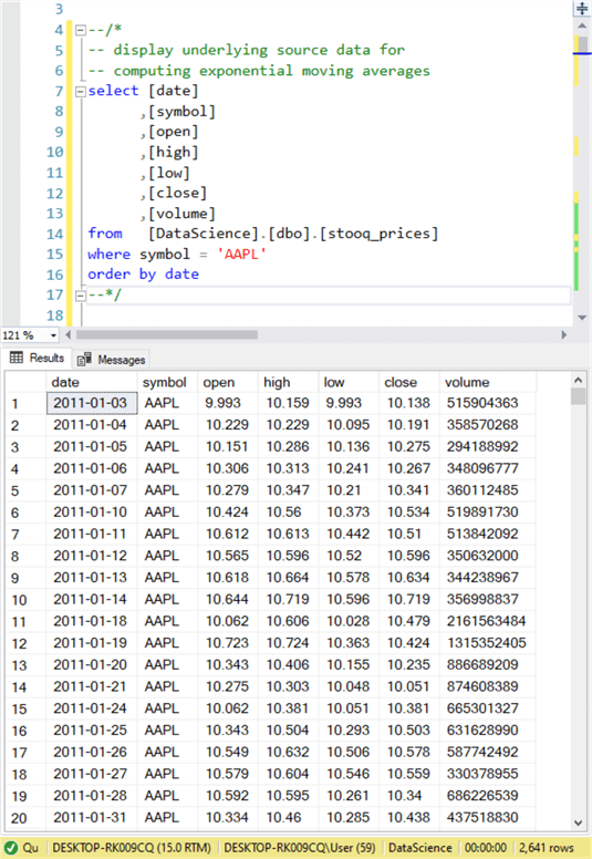
The following screen shot shows a simple query with sample time series data suitable for computing exponential moving averages. Key features of the data for exponential moving averages include

• The close column values for which exponential computing averages are normally computed
• The date column values which are the dates for which time series values are available. In this tip, the time series data extend from the first trading date in January 2011 through June 30, 2021.
• The symbol column values are all for AAPL in the following screen shot, but time series data are likely to include data for multiple symbols. In this tip, the stooq_prices table in the dbo schema of the DataScience database includes source data for six ticker symbols: AAPL, GOOGL, MSFT, SPXL, TQQQ, and UDOW.
• The other columns are useful for other use cases besides computing exponential moving averages.

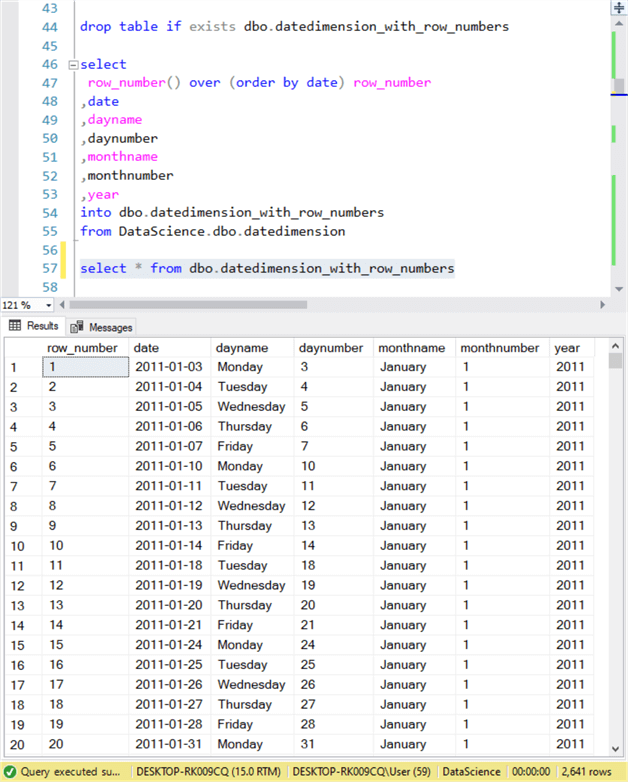
The next screen shot shows the sql for creating and listing the calendar table (dbo.datedimension_with_row_numbers) for this time series analysis. This calendar table is built on another previously created calendar table (dbo.datedimension). The modification in this example is to add a row_number calendar that assigns an int value to each row in the calendar. The original calendar table has a primary key of date with a sort order of date.

The image below shows all the trading dates in January 2011. There are just 20 dates in the trading calendar for January 2011 (see the row_number column). As you can see, some day numbers are missing.

• January 1 and 2 are weekend days when the US security markets are closed. The trading calendar table is also missing other weekend days in the month. US security markets are closed on weekend dates.
• In addition, Monday, January 17, 2011 is missing because this date is a US national holiday. The US securities markets are closed during a subset of the US national holidays.
• Because of missing weekend and holiday dates, the sequential order of trading dates does not match the sequential order of daily calendar dates. The row_number column makes it easy to track the order of trading dates.

The following script is for creating a table (emas_for_stooq_prices) for holding exponential moving average values. The table has five columns: row_number, date, symbol, ema_10 and ema_20. The last two columns are, respectively, for holding exponential moving averages with period lengths of 10 and 20. You can designate a separate column for each ema that you require.

The emas_for_stooq_prices table references the dates in the original calendar table on which the trading calendar table is also dependent. The first alter table adds a constraint to specify this dependence. The name of the constraint is fkey_date. The second alter table enables the constraint specified in the first alter table statement.

-- create a fresh version of the emas_for_stooq_prices table
drop table if exists dbo.emas_for_stooq_prices
 
-- create dbo.emas_for_stooq_prices table
create table dbo.emas_for_stooq_prices(
       row_number int NOT NULL,
   [date] [date] NOT NULL,
   [symbol] [nvarchar](10) NOT NULL,
   [ema_10] [money] NULL,
   [ema_20] [money] NULL,
) 
go
 
-- create foreign key reference to datedimension table
alter table dbo.emas_for_stooq_prices with nocheck add constraint [fkey_date] foreign key([date])
references dbo.datedimension ([date])
on update cascade
on delete cascade
go
 
-- enable foreign key constraint
alter table dbo.emas_for_stooq_prices check constraint fkey_date
go

There is one remaining table used in the process for computing exponential moving averages. This table named table_of_symbols tracks all the symbols in stooq_prices table of underlying time series values. Recall that ticker symbols partly identify a set of time series values. The table_of_symbols table contains a separate row for each distinct ticker symbol in the stooq_prices table. On each row, there is symbol_number identifier value and a string value for the symbol.

The following code excerpt illustrates an approach to creating a fresh copy of the table_of_symbols table with a row for each distinct ticker symbol in stooq_prices. The drop table if exists statement removes a prior table version if one already exists in the dbo schema of the default database. A nested pair of select statements pulls distinct symbols from stooq_prices in its inner query. The outer query uses the T-SQL row_number() function to assign a numeric identifier (symbol_number) for each distinct symbol. The into clause populates the table_of_symbols table with the results set from the outer query.

-- create a fresh version of the emas_for_stooq_prices table
drop table if exists dbo.table_of_symbols
go
 
-- populate table of symbols
select row_number() over (order by symbol) symbol_number, symbol
into dbo.table_of_symbols
from
(
   -- display distinct symbols in [DataScience].[dbo].[stooq_prices]
   select distinct symbol from [DataScience].[dbo].[stooq_prices]
) for_symbol_table
 
-- optionally, display table_of_symbols
-- select * from dbo.table_of_symbols

The T-SQL code for computing exponential moving averages

The code for computing the exponential moving averages relies on two nested while loops.

• The outer while loop iterates through each of the symbols in the table_of_symbols table. There are six distinct ticker symbols in the data for this tip. Therefore, the outer while loop operates six times.
• The inner while loop populates the emas_for_stooq_prices table rows with values corresponding to the underlying time series values (stooq_prices). In this tip, there are two exponential moving average values (ema_10 and ema_20) for each underlying close price value. There are also 2641 time series rows for each symbol. The inner loop operates 15,846 times across all six symbols (6 * 2641).

Before starting the while loops, the code for computing exponential moving averages declares a set of local variables and populates some of them for use on the first and/or all passes through the loops.

• The first three local variables (@symbol, @max_symbol_number, @symbol_index) are for managing passes through the outer while loop.
  • The @symbol_index local variable is for holding symbol_number column values from the table_of_symbols table on successive passes through the outer loop.
  • The @max_symbol_number local variable is populated with the maximum number of rows in the table_of_symbols table.
  • The @symbol local variable is the ticker symbol for the current pass through the outer loop.
• The remaining local variables were passing through close prices for the dates associated with each of the six symbols and computing ema_10 and ema_20 column values in the emas_for_stooq_prices table.

-- declare local variables 
declare
 @symbol nvarchar(10)
,@max_symbol_number int = (select max(symbol_number) from dbo.table_of_symbols)
,@symbol_index int = 1
,@alpha_10 float = 2.0/(10+1)
,@alpha_20 float = 2.0/(20+1)
,@current_row_number int = 3
,@max_row_number int = (select max(row_number) from datedimension_with_row_numbers)
,@xt money
,@ema_10_lag_1 money
,@ema_10 money
,@ema_20_lag_1 money
,@ema_20 money

The code for the while loops appears next.

• The outer while loop starts with a value for @symbol_index of 1 and increases its values by 1 on each successive pass through the outer while loop. The @max_symbol_number is the maximum number of distinct symbols in stooq_prices. When the value of @symbol_index exceeds @max_symbol_number control passes to the first statement after the outer while loop.
• The code inside the outer while loop starts by populating the first two rows in the emas_for_stooq_prices table for the symbol column value from the table_of_symbols on the row matching @symbol_index.
• After populating the first two rows in the emas_for_stooq_prices table for the current value of @symbol, the code uses the inner while loop to populate the remaining rows for the emas_for_stooq_prices table. The inner loop continues iterating until @current_row_number is greater than @max_row_number.
  • The @current_row_number local variable starts with a value of 3 (from the preceding declare statement).
  • On each pass through the inner while loop, the value of @current_row_number is incremented by 1.
  • When the value of @current_row_number exceeds @max_row_number all rows for the current symbol are processed and control passes to the first statement after the inner while loop.
• The main purpose of the inner while loop is to compute ema_10 and ema_20 for current row in the emas_for_stooq_prices table. Each step in this process is preceded by a brief comment indicating the role of the following code.
  • The process starts by retrieving the close value for the current row.
  • Next, the code retrieves ema_10 from the preceding row.
  • Then, the code computes the exponential moving average with a period length of 10 and saves the result in @ema_10.
  • Next the code retrieves ema_20 from the preceding row.
  • Then, the code computes the exponential moving average with a period length of 20 and saves the result in @ema_20.
  • The final step for adding a new row of ema values is to insert @ema_10 and @ema_20 into emas_for_stooq_prices for the current row.
• When control passes from the inner loop to the outer loop, the values of @symbol_index and @current_row_number are updated for the next ticker symbol (if there is one remaining) to be processed.

-- while loop for iterating through symbols
while @symbol_index <= @max_symbol_number
begin
 
   -- assign a fresh value to @symbol from table_of_symbols
   select @symbol = symbol from table_of_symbols where symbol_number = @symbol_index
 
   -- populate first two rows in emas_for_stooq_prices
   insert into dbo.emas_for_stooq_prices
   (
    symbol
   ,date
   ,row_number
   ,ema_10
   ,ema_20
   )
   --*/
   -- values for first two rows in dbo.emas_for_stooq_prices
   select 
    symbol
   ,date
   ,case
      when rn = 1 then 1
      when rn = 2 then 2
    end row_number
   ,case
      when rn = 2 then lag([close],1) over (order by date)
    end ema_10
   ,case
      when rn = 2 then lag([close],1) over (order by date)
    end ema_20
   from
   (
   -- rn, symbol, date, close 
   select 
    row_number() over (order by stooq_prices.date) rn
   ,@symbol symbol
   ,stooq_prices.date
   ,[close]
   from dbo.datedimension
   inner join dbo.stooq_prices
   on stooq_prices.date = datedimension.date
   where stooq_prices.symbol = @symbol
   ) for_priming_
   where rn <= 2
 
   -- optionally, display top two rows from emas_for_stooq_prices
   -- select * from dbo.emas_for_stooq_prices
 
   -- compute exponential moving averages for
   -- all remaining underlying source data rows
   while @current_row_number <= @max_row_number
   begin
 
      -- retrieve close value (@xt) for @current_row_number
      set @xt = (select [close]
      from dbo.datedimension_with_row_numbers
      join dbo.stooq_prices on datedimension_with_row_numbers.date = stooq_prices.date
      where datedimension_with_row_numbers.row_number = @current_row_number and stooq_prices.symbol = @symbol)
 
      -- retrieve ema_10 for prior row
      set @ema_10_lag_1 =(select ema_10
      from dbo.datedimension_with_row_numbers
      --join dbo.stooq_prices on datedimension_with_row_numbers.date = stooq_prices.date
      join dbo.emas_for_stooq_prices on datedimension_with_row_numbers.date = emas_for_stooq_prices.date
      where datedimension_with_row_numbers.row_number = (@current_row_number-1) and emas_for_stooq_prices.symbol = @symbol)
 
      -- compute ema_10 for @current_row_number
      set @ema_10 = (@alpha_10*@xt) + ((1-@alpha_10)*@ema_10_lag_1)
 
      -- retrieve ema_20 for prior row
      set @ema_20_lag_1 =(select ema_20
      from dbo.datedimension_with_row_numbers
      --join dbo.stooq_prices on datedimension_with_row_numbers.date = stooq_prices.date
      join dbo.emas_for_stooq_prices on datedimension_with_row_numbers.date = emas_for_stooq_prices.date
      where datedimension_with_row_numbers.row_number = (@current_row_number-1) and emas_for_stooq_prices.symbol = @symbol)
 
      -- compute ema_20 for @current_row_number
      set @ema_20 = (@alpha_20*@xt) + ((1-@alpha_20)*@ema_20_lag_1)
 
      -- insert row into emas_for_stooq_prices for @current_row_number
      insert into dbo.emas_for_stooq_prices
      (
       row_number
      ,symbol
      ,date
      ,ema_10
      ,ema_20
      )
      select 
       @current_row_number
      ,@symbol symbol
      ,(
         select [date]
         from dbo.datedimension_with_row_numbers
         where datedimension_with_row_numbers.row_number = @current_row_number
         ) date
      ,@ema_10
      ,@ema_20
 
      -- set @current_row_number for next while condition criterion
      set @current_row_number = @current_row_number + 1
 
   end
 
   set @symbol_index = @symbol_index + 1
   set @current_row_number = 3
end
 
-- display first ten rows from emas_for_stooq_prices
   select * from dbo.emas_for_stooq_prices where row_number <=10 order by symbol, row_number
 
-- display last ten rows from emas_for_stooq_prices
   select * from dbo.emas_for_stooq_prices where row_number >= (@max_row_number-9)  order by symbol, row_number
 
-- optionally, display all from emas_for_stooq_prices
   --select * from dbo.emas_for_stooq_prices order by symbol, row_number

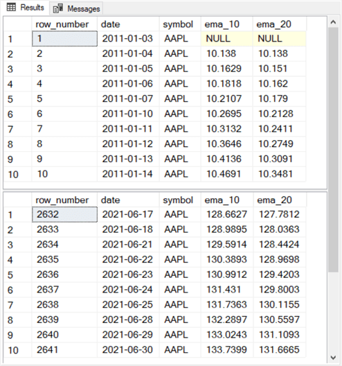
Here is a screen shot with the first and last ten rows from the emas_for_stooq_prices table from the preceding script excerpt.

A look at the log table from a SQL Server model for time series data

A use case for emas is to compare two or more emas with different period lengths versus one another for specifying when to buy and sell financial securities. When an ema with a shorter period length exceeds another ema with a longer period length, then the underlying time series values are increasing on average. In contrast, when an ema with a shorter period length is less than or equal to another ema with a longer period length, then the underlying time series data are declining on average.

Based on these two relationships, you can detect reversals between two contiguous periods in the underlying time series values. If you are able to buy a financial security shortly after it reverses from a falling to a rising trend, then you may be able to sell the security shortly after it reverses again from a rising trend to a falling trend. This section introduces some T-SQL code that allows you to compute profitability of this reversal detection strategy with historical data.

• The following code excerpt specifies two criteria for assigning a buy signal string value or a sell signal value to a buy_sell_signal column value
  • in the current period, when the ema with a shorter period length (ema_10) is greater than another ema with a longer period length (ema_20) and
  • in the preceding period, when the ema with a shorter period length (ema_10_lag_1) is less than or equal to the ema with a longer period length (ema_30_lag_1)
  • then assign a buy signal string value to the current row of the buy_sell_signal column because this points to a reversal from falling to rising security prices.
• When the criteria are reversed as in the second when clause of the first case statement, then assign a sell signal value to the current row of the buy_sell_signal column because this identifies a reversal from rising to falling security prices.
• Likewise, the case statement code for assigning buy_sell_price column values assigns buy and sell prices based on the same criteria used for assigning buy signal and sell signal string values to the buy_sell_signal column.
  • Because you cannot know ema values for close prices until after a trading day closes, a buy_sell_signal column value points to a buy action or a sell action for the next trading day
  • Therefore, the buy_sell_price column value for the next trading day is based on the preceding trading day’s buy_sell_signal column value. The reversal specifies an action (buy or sell) for the next trading day
  • You can get the next row’s open price with a SQL Server lead function. A lead function in other code preceding the excerpt below populates the open_lead_1 column in the source data for the code excerpt below

-- set buy and sell signals
,case
   when ((ema_10_lag_1 <= ema_30_lag_1) and  (ema_10 > ema_20)) then 'buy signal'
   when ((ema_10_lag_1 >= ema_30_lag_1) and (ema_20 > ema_10)) then 'sell signal'
   else null
 end buy_sell_signal
 
-- set buy and sell prices
,case
   when ((ema_10_lag_1 <= ema_30_lag_1) and  (ema_10 > ema_20)) then open_lead_1
   when ((ema_10_lag_1 >= ema_30_lag_1) and (ema_20 > ema_10)) then open_lead_1
   else null
 end buy_sell_price

The full query statement that includes the preceding excerpt appears is in this prior tip Assessing Time Series Model Performance with T-SQL. The full query statement writes a log of rows with the computed buy_sell_signal and buy_sell_price column values. Each log contains multiple buy-sell cycles that depend on the criteria, such as those appearing in the preceding excerpt. Each buy-sell cycle starts with the row after a buy signal and continues through the first row after the next sell signal.

• The log typically contains an alternating list of buy signals and sell signals.
• However, it can also happen that there are multiple buy signals from the first buy signal in a buy-sell cycle through the first sell signal in buy-sell cycle.
• Likewise, after the first sell signal trailing a buy signal that starts a buy-sell cycle, there can be one or more rows with sell signals before the start of a new buy-sell cycle based on a buy signal that trails the preceding buy-sell cycle.

Between successive buy-sell cycles, there can be a variable number of rows depending on the source data and the criteria for determining when a row should have either a buy signal or a sell signal. Furthermore, the number of rows or time periods in a buy-sell cycle can vary from one buy-sell cycle to the next. The only reliable landmarks that you have in the log of buy-sell cycles are

• The buy signal and sell signal for the first buy-sell cycle or the buy signal and sell signal from the preceding buy-sell cycle depending on which buy-sell cycle is more recent
• The buy signal and sell signal from the current buy-sell cycle

By walking through successive buy-sell cycles in a log and monitoring the flow of buy signals and sells signals from the most recently completed buy-sell cycle, you can specify when the next buy-sell cycle will start and end. For example, the next buy-sell cycle cannot start until after the preceding buy-sell cycle ends. In like manner, the current buy-sell cycle must end after the start of the current buy-sell cycle.

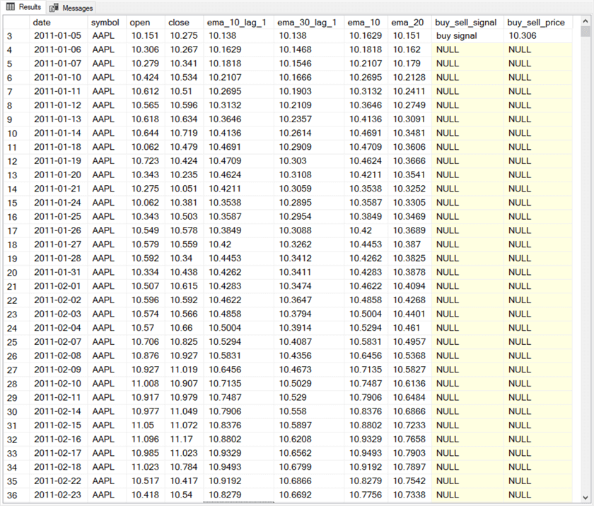
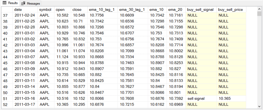
The following pair of screen shots show the beginning and end of a buy-sell cycle with a single starting buy signal row and ending with a single sell signal row. The buy-sell cycle starts with the row after the buy signal and runs through the first row trailing sell signal row.

• The first screen image starts with the buy signal on 2011-01-05 that precedes the first buy action on 2011-01-06. The first screen shot ends on 2011-02-23. This is just for formatting purposes.
• The second screen image continues from 2011-02-24 and ends on 2011-03-17. The final date (2011-03-17) is when the sell action executes because of the sell signal on 2011-03-16.
• The buy-sell cycle in the following pair of screen images starts on the trading day after the buy signal row and ends on the trading day after the sell signal row.

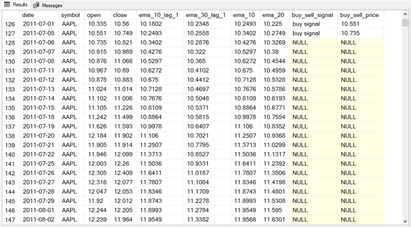
The next pair of screen shots show the log rows for a buy-sell cycle containing more than one buy signal. The log for the buy-sell cycle also show a pair of sell signals after the sell signal that points to the sell action row that ends the buy-sell cycle.

• The buy signal row on 2011-07-01 is for the trading day that recommends a buy action for the buy-sell cycle. The buy action for the buy-sell cycle is on 2011-07-05, the first trading day after the buy signal row.
• Notice that buy_sell_signal column also has a buy signal on 2011-07-05. However, this second buy signal does not recommend a buy action because the security is already bought.
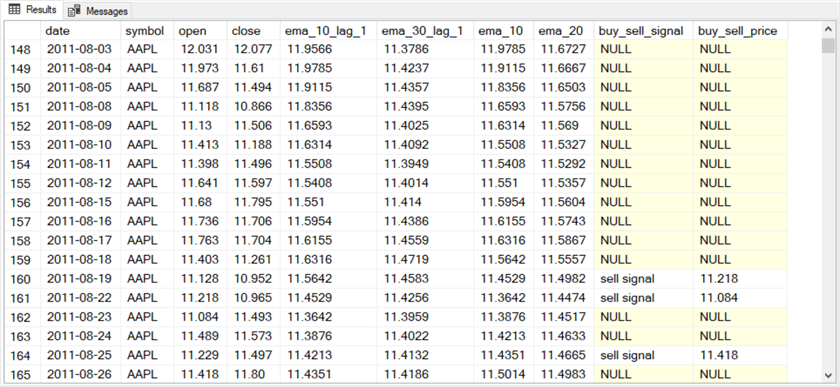
• The sell signal row on 2011-08-19 recommends a sell action to end the buy-sell cycle on 2011-08-22. Therefore, the buy-sell cycle ends on 2011-08-22.
• Despite the fact that the buy-sell cycle ends on 2011-08-22, the second screen shot in the pair below shows two additional sell signal rows without an intervening buy signal row. This is not an error. It is just the kind of behavior that routinely happens with time series data. In any event, once a buy-sell cycle ends additional sell signals without an intervening buy signal do not cause the model to recommend that you should sell the security again.

As the preceding screen shots show, it is easy to have buy signal and sell signal rows in time series data that do not necessarily recommend any action from a model. Code for compiling start and end dates for buy-sell cycles from a log table needs to distinguish between buy signal and sell signal rows that recommend an action from those that do not. The following script demonstrates how to use a goto statement inside an if…else statement to navigate through a log table and extract the start and end dates for a series of buy-sell cycles. This kind of action is required as a first step to compute the gain or loss associated for each buy-sell cycle.

T-SQL code for deriving buy-sell cycle dates for a symbol from a log table

The log table from the preceding section has a row for each date from the first date through the last date in a test dataset for evaluating a model that recommends when to buy and sell securities for a ticker symbol. This tip uses a test dataset that has its first trading date at the beginning of January in 2011 and runs through June 30, 2021. The dataset also has a separate set of log rows for each of six ticker symbols: AAPL, GOOGL, MSFT, SPXL, TQQQ, UDOW.

The code is for extracting a set of buy signal dates with matching sell signal dates for a ticker symbol from a log table. The code relies on six local variables for tracking dates associated with the first buy-sell cycle for a ticker symbol and then each subsequent buy-sell cycle for a ticker symbol.

The following code excerpt declares the local variables and extracts the subset of log rows for a designated ticker symbol. The excerpt starts with the a declare statement for seven local variables.

• @symbol is for the ticker symbol for which buy-sell cycle dates will be compiled. In the excerpt below, this local variable is set to the AAPL ticker symbol.
• @first_buy_signal_date and @first_sell_signal_date local variables are, respectively, for the first buy signal and the first sell signal date for a ticker symbol.
• @prior_buy_signal_date and @prior_sell_signal_date local variables are, respectively, for the buy signal and sell signal dates for the preceding buy-sell cycle.
• @next_buy_signal_date and @next_sell_signal_date local variables are, respectively, for the buy signal and sell signal dates for the next buy-sell cycle.

The second part of the excerpt below performs a subset from the log table (log_for_buy_at_ema_10_gt_20) for the rows belonging to the current @symbol value; the subset table is assigned the name symbol_temp_log. Additionally, the second part adds a new set of column values to the subset table that are not in the full log. The new column has the name next_date. The value for this column is the date column value of the next row in the log table.

-- declarations
declare 
    @symbol nvarchar(10) = 'AAPL'
   ,@first_buy_signal_date date
   ,@first_sell_signal_date date
   ,@prior_buy_signal_date date
   ,@prior_sell_signal_date date
   ,@next_buy_signal_date date
   ,@next_sell_signal_date date
 
-- create and populate a temp log for a symbol 
-- with buy_sell_signal dates (next_date)
drop table if exists dbo.symbol_temp_log
 
select [date]
      ,[symbol]
      ,[open]
      ,[close]
      ,[ema_10_lag_1]
      ,[ema_30_lag_1]
      ,[ema_10]
      ,[ema_20]
      ,[buy_sell_signal]
      ,[buy_sell_price]
      ,lead(date,1) over (partition by symbol order by date) next_date
into dbo.symbol_temp_log
from   [DataScience].[dbo].[log_for_buy_at_ema_10_gt_20]
where symbol = @symbol

The primary role for the next code excerpt is to create a table for saving buy and sell dates associated with buy-sell cycles in a log table. The code also populates the table with buy and sell dates for the first buy-sell cycle, and it assigns values to the @prior_buy_signal_date and @prior_sell_signal_date local variables. The @prior_sell_signal_date local variable value serves as a reference point for computing the beginning of the second buy-sell cycle.

• The first two statements at the top of the script create a fresh version of the symbol_buy_sell_cycle_date table; the table has two columns
  • One column is for the current value of @symbol
  • The other column saves buy signal and sell signal dates for successive buy-sell cycles.
• Next, a pair of set statements assign the first buy signal date to @first_buy_signal_date and the first sell signal date to @first_sell_signal_date
• Then, the first two rows of the symbol_buy_sell_cycle_date table are populated for the first buy-sell cycle
• The following excerpt closes by assigning
  • @first_buy_signal_date to @prior_buy_signal_date
  • @first_sell_signal_date to @prior_sell_signal_date
• The assignment for @prior_buy_signal_date is to configure it for searching for the first buy signal date for the next buy-sell cycle

drop table if exists dbo.symbol_buy_sell_cycle_date
 
create table dbo.symbol_buy_sell_cycle_date(
    [symbol] [nvarchar](10) not NULL
   ,[buy_sell_cycle_date] [date] NOT NULL,
)
 
-- compute @first_buy_signal_date and @first_sell_signal_date
-- and insert into dbo.symbol_buy_sell_cycle_date
 
set @first_buy_signal_date = (select min(next_date) 
from symbol_temp_log
where buy_sell_signal = 'buy signal')
 
set @first_sell_signal_date = (select min(next_date)
from symbol_temp_log
where buy_sell_signal = 'sell signal')
 
insert dbo.symbol_buy_sell_cycle_date
select *
from
(
select @symbol [symbol], @first_buy_signal_date [buy_sell_cycle_date]
union
select @symbol [symbol], @first_sell_signal_date [buy_sell_cycle_date]
) buy_sell_cycle_dates
 
set @prior_buy_signal_date = @first_buy_signal_date
set @prior_sell_signal_date = @first_sell_signal_date

The final code excerpt in this section searches through the log table to find start and end dates for successive buy-sell cycles after the first buy-sell cycle. The code saves each discovered start and end date in the symbol_buy_sell_cycle_date table. It achieves this goal by iteratively detecting the start of a new buy-sell cycle from the end of a preceding buy-sell cycle. Given the start date for a new buy-sell cycle, the code searches for the end of the new buy-sell cycle. An if…else statement either saves the current @next_buy_signal_date and @next_sell_signal_date local variables values in the symbol_buy_sell_cycle_date table or ceases searching because there are no additional buy-sell cycles to be found.

• To continue searching, the Boolean expression in the if clause must discover that neither the buy date nor the sell date is null for the prospective new buy-sell cycle.
• The if branch starts by populating symbol_buy_sell_cycle_date table with the buy and sell dates for a new cycle. After this, a goto statement loops back to the Next_Buy_Sell_Pair label statement at the top of the excerpt to continue searching for the start and end dates of another buy-sell cycle.
• The else branch executes when there are no more buy-sell cycles in the log table. Some commented code can be uncommented to optionally display the contents of the symbol_buy_sell_cycle_date table. A return statement in the else clause transfers control to the first statement after the if…else statement.

-- after search for @first_buy_signal_date and @first_sell_signal_date
-- search iteratively for @next_buy_signal_date and @next_sell_signal_date
 
Next_Buy_Sell_Date_Pair:
set @next_buy_signal_date = (select min(next_date) next_buy_signal_date
from symbol_temp_log 
where buy_sell_signal = 'buy signal' and next_date > @prior_sell_signal_date)
 
set @next_sell_signal_date = (select min(next_date) next_sell_signal_date 
from symbol_temp_log
where buy_sell_signal = 'sell signal' and next_date > @next_buy_signal_date)
 
-- assign @next_buy_signal_date and @next_sell_signal_date
-- to @prior_buy_signal_date and @prior_buy_signal_date
-- for next iterative search if another search is needed
set @prior_buy_signal_date = @next_buy_signal_date
set @prior_sell_signal_date = @next_sell_signal_date
 
 
-- cease searching iteratively when at least one null date value is returned 
-- when no null returned, then insert cycle dates into symbol_buy_sell_cycle_date table
if @next_buy_signal_date is not null and @next_sell_signal_date is not null
begin
 
   insert dbo.symbol_buy_sell_cycle_date
   select *
   from
   (
   select @symbol [symbol], @next_buy_signal_date [buy_sell_cycle_date]
   union
   select @symbol [symbol], @next_sell_signal_date [buy_sell_cycle_date]
   ) buy_sell_cycle_dates
 
   goto Next_Buy_Sell_Date_Pair
 
end
else 
begin
   
   -- optionally display symbol_buy_sell_cycle_date table
   -- after all buy_sell cycle dates are discovered 
   -- for the current symbol
   -- select * from dbo.symbol_buy_sell_cycle_date
 
      return 
end

The symbol_buy_sell_cycle_date table is useful for computing current balance over successive buy-sell cycles. By computing current balance over successive buy-sell cycles, additional code can reveal the relative success of different models for growing an initial investment over successive trades.

Next Steps

This tip illustrates two appropriate use cases for iterative development techniques with time series data. Some time series requirements call for computing or extracting current values based on antecedents. You can recognize these use cases and other use cases as appropriate for iterative development techniques because you are computing or compiling new row values that cannot be known until after prior row values become computed or compiled.

Because SQL Server applications typically rely on observations instead of computed or compiled values from prior rows, set-based approaches are almost always the best way to perform data manipulations. However, with some time series applications, that is not necessarily the case. After iterative techniques are used to compute or compile a set of time series values, then set-based approaches can be appropriate for referencing the values derived by iterative techniques.

For those who want to try some of the programming techniques discussed in this tip, there are four files in the tip’s download.

• While_loop_time_series_example_try_1.sql contains the T-SQL script for computing exponential moving averages.
• stooq_prices.csv contains a csv file with the data for stooq_prices table. Import and copy stooq_prices.csv into a SQL Server table and reference the table with the preceding script.
• Goto_demo_for_buy_sell_start_and_end_cycles.sql contains the T-SQL script for computing start and end dates for buy-sell cycles for each of six ticker symbols.
• log_for_buy_at_ema_10_gt_20.csv contains the data for the log_for_buy_at_ema_10_gt_20 table. Import and copy log_for_buy_at_ema_10_gt_20.csv into a SQL Server table and reference the table with the preceding script.

About the author

Rick Dobson is an author and an individual trader. He is also a SQL Server professional with decades of T-SQL experience that includes authoring books, running a national seminar practice, working for businesses on finance and healthcare development projects, and serving as a regular contributor to MSSQLTips.com. He has been growing his Python skills for more than the past half decade -- especially for data visualization and ETL tasks with JSON and CSV files. His most recent professional passions include financial time series data and analyses, AI models, and statistics. He believes the proper application of these skills can help traders and investors to make more profitable decisions.

This author pledges the content of this article is based on professional experience and not AI generated.

View all my tips