Assessing Time Series Model Performance with T-SQL

By: Rick Dobson   |   Updated: 2022-02-02   |   Comments (1)   |   Related: > TSQL

Problem

A prior pair of tips compared the performance of time series models based on exponential moving average crossovers. The models issued recommendations about when to buy and sell securities. Please review the T-SQL code for implementing each model. Also, present and compare analytical frameworks that assess the performance to accumulate gains for models recommending when to buy and sell securities.

Solution

A prior pair of tips (here and here) introduces T-SQL developers to formulating and comparing time series models based on exponential moving average crossovers. This kind of model is an example of artificial intelligence in the sense that a model issues a recommendation about when to perform an action instead of a human making a recommendation. One especially early use case for artificial intelligence was recommending moves in chess games. More recently, artificial intelligence has a much broader range of use cases, such as facial recognition and inventory management.

One way to enhance artificial intelligence models is by tracking the performance of model design changes. Even just assessing two model designs can help you to pick the best design for future refinement. When working with artificial intelligence for recommendations about financial decisions, a valid assessment strategy is comparing the returns from each of two models. This design approach will help you pick a set of code to which you can add more features to improve future recommendations from your AI models.

This tip has two objectives. First, it presents and describes T-SQL code for artificial intelligence models that recommend when to buy and sell financial securities. Related points include tracking the recommendations and their performance over time. Second, the tip highlights different techniques for aggregating the returns from a succession of trades recommended by the models for individual securities as well as a portfolio of securities. The source data for the tip tracks six financial securities (AAPL, GOOGL, MSFT, SPXL, TQQQ, and UDOW) over a 10.5 year interval (from January 2011 through June 30, 2021).

T-SQL for a pair of AI models

The following script excerpt illustrates core T-SQL coding techniques for writing buy and sell signals and prices to a log for an artificial intelligence model. The following code is for one of the two models examined in this tip. The T-SQL script files for the models (along with other supporting files) are in the tip’s download.

• Both models store successive trade recommendations in a log table named log_for_buy_at_ema_10_gt_20 table in the DataScience database.
• This following script excerpt is from the log_cleaning_for_rising_and_falling_below_20_ema_revised_for_prior_at_ema_20.sql file. The model for this script file is referred to as the first model throughout this tip.
• Two case statements in the select list items write buy and sell signals with their associated prices to the log.
• Additional select items post exponential moving averages used by the model to make recommendations.
• Because the code is for a time series model, the order of the rows based on dates is particularly important.
  • The ema_10 and ema_20 column values represent, respectively, ten-period length and twenty-period length exponential moving averages computed for the close price of a security on the current row.
  • The ema_10_lag_1 and ema_20_lag_1 column values denote, respectively, ten-period length and twenty-period length exponential moving averages computed for the close price of the prior row. The model uses the SQL Server lag function to compute ema_10_lag_1 and ema_20_lag_1 column values.
  • You cannot know the close price for a security on a trading date until after the close of trading that day.
  • The buy and sell actions recommended by the model are for execution on the trading date after the current trading date. The prices on the execution dates are in the open_lead_1 column. The open price is the first price on a trading date. The model uses the SQL Server lead functions to compute open_lead_1 column values, which represent the open price on the next trading date.
• Financial securities are denoted by ticker symbols in the source data. For example, MSFT is the symbol for Microsoft corporation common stock, and AAPL is for Apple corporation common stock.
• The into clause before the from clause in the select statement saves the buy_sell_signal and buy_sell_price computed columns along with selected other columns to the log table. The log persists recommended actions and their model outcomes.

Notice that the following script derives its column values for the outer query from a subquery named for_buy_sell_log_for_ema_10_vs_20. The subquery returns

• all columns from the stooq_prices table, which contains information for symbols, close prices, and open prices on successive trading dates
• selected columns from the denormalized_emas table, which contains exponential moving averages for different symbols on successive trading dates
• three computed columns named
  • ema_10_lag_1
  • ema_20_lag_1
  • open_lead_1

The computed columns in the subquery derive from SQL Server window aggregate functions. You can learn more about SQL Server window aggregate functions from this MSSQLTips.com tutorial. If you do not have the tables on your SQL Server referenced by the subquery, then import a csv file with the source data from this tip’s download. Then replace the reference to the subquery with a reference to the SQL Server table holding the contents of the imported csv file.

Just because there is a buy signal or sell signal in a log row does not mean that the model necessarily recommends a buy action or a sell action. This is because after the first buy price in a buy-sell cycle, there may be one or more other rows that satisfy the criteria for a buy signal before the sell signal row corresponding to the initial buy signal row in a buy-sell cycle. Similarly, after the first sell signal row following a buy signal row, there can be one or more additional sell signal rows before the next buy signal.

use [DataScience]
go
 
-- create the log for all symbols
drop table if exists dbo.log_for_buy_at_ema_10_gt_20
 
-- create dbo.log_for_buy_at_ema_10_gt_20
select 
   date
  ,symbol
  ,[open]
  ,[close]
  ,ema_10_lag_1
  ,ema_20_lag_1
  ,ema_10
  ,ema_20
  -- set buy and sell signals
  ,case
     when ((ema_10_lag_1 <= ema_20_lag_1) and  (ema_10 > ema_20)) then 'buy signal'
     when ((ema_10_lag_1 >= ema_20_lag_1) and (ema_20 > ema_10)) then 'sell signal'
     else null
     end buy_sell_signal
   -- set buy and sell prices
  ,case
     when ((ema_10_lag_1 <= ema_20_lag_1) and  (ema_10 > ema_20)) then open_lead_1
     when ((ema_10_lag_1 >= ema_20_lag_1) and (ema_20 > ema_10)) then open_lead_1
     else null
     end buy_sell_price
 
into dbo.log_for_buy_at_ema_10_gt_20

from 
( 
  -- source rows for buy/sell actions 
  select 
     stooq_prices.* 
    ,denormalized_emas.ema_10 
    ,denormalized_emas.ema_20 
    ,denormalized_emas.ema_30 
    ,denormalized_emas.ema_50 
    ,lag(denormalized_emas.ema_10,1) over (partition by stooq_prices.symbol order by denormalized_emas.date) ema_10_lag_1 
    ,lag(denormalized_emas.ema_20,1) over (partition by stooq_prices.symbol order by denormalized_emas.date) ema_20_lag_1 
    ,lead(stooq_prices.[open],1) over(partition by stooq_prices.symbol order by denormalized_emas.date) open_lead_1 
  from DataScience.dbo.stooq_prices 
  inner join DataScience.dbo.denormalized_emas 
     on stooq_prices.date = denormalized_emas.date 
     and stooq_prices.symbol = denormalized_emas.symbol 
) for_buy_sell_log_for_ema_10_vs_20 

The next script excerpt is from the log_cleaning_for_rising_and_falling_below_20_ema_revised_for_prior_at_ema_30.sql file in the download for this tip found at the end. The model for this script file is referred to as the second model throughout this tip.

• When writing a buy signal in a row,
  • the preceding query requires that the ema_10 be less than or equal to ema_20 in the prior row relative to the current row (ema_10_lag_1 <= ema_20_lag_1)
  • the following query requires that the ema_10 be less than or equal to ema_30 in the prior row relative to the current row (ema_10_lag_1 <= ema_30_lag_1)
• On the other hand, when writing a sell signal row,
  • The preceding query requires that the ema_10 be greater than or equal to ema_20 in the prior row relative to the current row (ema_10_lag_1 >= ema_20_lag_1)
  • The following query requires that the ema_10 be greater than or equal to ema_30 in the prior row to the current row (ema_10_lag_1 >= ema_30_lag_1)
• Because of the difference in criteria between the two queries, different results set values need to be passed from the subquery to the outer query. A separate csv file with values from each subquery is included in this tip’s download.

The current row criteria for buy signals are the same in the preceding and following queries. The criteria expression is: ema_10 > ema_20.

Also, the current row criteria for sell signals are the same in the preceding and following queries. The criteria expression is ema_20 > ema_10.

This mix of criteria expressions aims to detect trend reversals. The reason for evaluating two different models is to discover which criteria set is better at detecting trend reversals.

use [DataScience]
go
 
-- create the log for all symbols
drop table if exists dbo.log_for_buy_at_ema_10_gt_20
 
-- create dbo.log_for_buy_at_ema_10_gt_20
select 
   date
  ,symbol
  ,[open]
  ,[close]
  ,ema_10_lag_1
  ,ema_30_lag_1
  ,ema_10
  ,ema_20
  -- set buy and sell signals
  ,case
     when ((ema_10_lag_1 <= ema_30_lag_1) and  (ema_10 > ema_20)) then 'buy signal'
     when ((ema_10_lag_1 >= ema_30_lag_1) and (ema_20 > ema_10)) then 'sell signal'
     else null
     end buy_sell_signal
  -- set buy and sell prices
  ,case
     when ((ema_10_lag_1 <= ema_30_lag_1) and  (ema_10 > ema_20)) then open_lead_1
     when ((ema_10_lag_1 >= ema_30_lag_1) and (ema_20 > ema_10)) then open_lead_1
     else null
     end buy_sell_price
 
into dbo.log_for_buy_at_ema_10_gt_20
 
from
(
  -- source rows for buy/sell actions
  select 
     stooq_prices.* 
    ,denormalized_emas.ema_10
    ,denormalized_emas.ema_20
    ,denormalized_emas.ema_30
    ,denormalized_emas.ema_50
  --,denormalized_emas.ema_200
    ,lag(denormalized_emas.ema_10,1) over (partition by stooq_prices.symbol order by denormalized_emas.date) ema_10_lag_1
    ,lag(denormalized_emas.ema_30,1) over (partition by stooq_prices.symbol order by denormalized_emas.date) ema_30_lag_1
    ,lead(stooq_prices.[open],1) over(partition by stooq_prices.symbol order by denormalized_emas.date) open_lead_1
  from DataScience.dbo.stooq_prices
  inner join DataScience.dbo.denormalized_emas
     on stooq_prices.date = denormalized_emas.date
     and stooq_prices.symbol = denormalized_emas.symbol
) for_buy_sell_log_for_ema_10_vs_20

Examining the AI time series model logs

The core idea around each of the preceding time series models is that it may be a good time to buy a financial security right after its close prices reverse from going down to going up and sell a financial security right after its close prices reverse from going up to going down. The two models in the preceding section takes two slightly different paths to implementing this core idea.

• The first model assumes underlying close prices start to reverse and increase when ema_10 rises above ema_20 from a preceding day in which ema_20 is greater than or equal ema_10. This is the date for a buy signal date from the first model.
• The model in the log_cleaning_for_rising_and_falling_below_20_ema_revised_for_prior_at_ema_30.sql file assumes underlying close prices start to reverse and increase when ema_10 rises above ema_20 from a preceding day in which ema_30 is greater than or equal ema_10. This is the date for a buy signal date from the second model.
• The difference between the models is that the second model uses a longer period length for its longer-period-length ema.
• Let’s look at the model log and see the buy-sell recommendations that come from each model. For presentation purposes, the log rows were copied from SSMS to a tab in an Excel worksheet.

Here are three excerpts from the log for the AAPL ticker symbol from the first model. In the first two hundred log rows there are six buy-sell cycles, but just the first three are shown in this tip to familiarize you with the layout of the log.

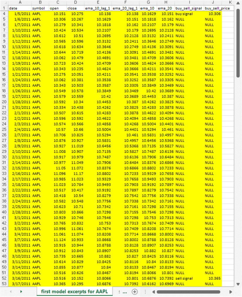
The following screen shows the log rows associated with the first buy-sell cycle from the first model. The worksheet tab indicates the display is from the first model for the AAPL ticker symbol.

• Row 1 shows the column headers.
• The buy signal occurs in row 4 of the buy_sell_signal column.
• The buy price shows in row 4 of the buy_sell_price column. Notice that the buy price on row 4 matches the open column value in row 5. Recall that this is because the execution of the action recommended by a buy signal occurs one trading date after the buy signal.
• The sell signal appears in row 52 of the buy_sell_signal column.
• The sell price also shows in row 53 of the open column. This is because the sell signal executes one trading date after the sell signal.
• The change in price during the first buy-sell cycle is 10.365, the open price on 3/17/2011, less 10.306, the open price on 1/6/2011.
• The number of trading days in the first buy-sell cycle commences with row 5 and goes through row 53 for a total of 49 trading dates.

The following screen shows the log rows associated with the second buy-sell cycle from the first model.

• The layout for showing the log rows from the second buy-sell cycle are the same as in the first buy-sell cycle.
• However, the duration of the second buy-sell cycle is dramatically shorter than for the first buy-sell cycle.
  • The number of trading days in the second buy-sell cycle is just 4 trading days.
  • The number of trading days in the first buy-sell cycle is more than 12 times greater – namely, 53 trading days.
• The reason the duration of the second buy-sell cycle is so much shorter than the first buy-sell cycle is that the sell signal is on the third trading day after the buy signal.
• This short duration is a good outcome.
  • The open price (10.657) on 3/31/2011 which is the buy price.
  • By 4/4/2011, the date for the sell signal in the second buy-sell cycle, the open price falls below the buy price.
  • The display below shows the open price falls even further below the buy price on 4/5/2011, which is the date for executing the recommended sell action for the second buy-sell cycle.
  • Furthermore, the worksheet with the first 200 log rows, which is available in this tip’s download, shows that open prices for successive trading days remain below the buy price through 4/20/2011.

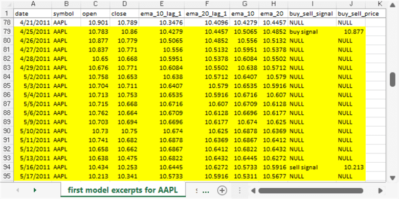
The following screen shows the log rows associated with the third buy-sell cycle from the first model. The rows with a yellow background are from the buy signal date through the date after the sell signal date.

• The row with a white background, for 4/21/2011, has an open price that reverses the close price declines from the preceding buy-sell cycle and rows after it as well.
• Then, after the end of the next trading day (4/25/2011), the first model issues a buy signal.
• The buy in response to the 4/25/2011 buy signal occurs at the open price on 4/26/2011.
• The third buy-sell cycle remains in effect through the trading day after 5/17/2011. As you can see in the log, a sell signal is issued on 5/16/2011 after the close of trading. Then, a sell occurs at the open of the next trading day (5/17/2011).
• Just like the second buy-sell cycle, the log reveals a loss. The loss per share is the sell price of 10.213 less the buy price of 10.877.

Two of the first three buy-sell cycles from the first model resulted in losses.

Here are four excerpts from the log for the AAPL ticker symbol from the second model. In the first two hundred log rows, there are six buy-sell cycles. However, this tip examines just the first four buy-sell cycles because the format of those log rows is sufficient to reveal special layout issues of the log rows from the second model and reinforce your understanding of log layouts from either model.

Recall that the difference between the first and second models is in the emas compared to ascertain if underlying close prices were rising or falling through the prior period to the current trading date.

• In the first model, ema_10 is compared to ema_20 in the prior period.
• In the second model, ema_10 is compared to ema_30 in the prior period.
• Because ema_10 is closer to ema_20 than ema_30, the ema_10 has to fall more in the second model than the first model.
• Also, because both models base a rising price trend on the same two emas (ema_10 and ema_20), the reversal in price trends for the second model is greater than for the first model.

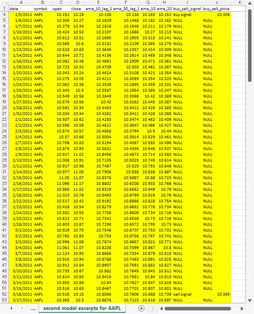
The following screen shows the log rows associated with the first buy-sell cycle from the second model. The worksheet tab confirms the display is from the second model for the AAPL ticker symbol. Although the log rows shown below are from the second model, the resulting log rows exactly match those from the first model for its first buy-sell cycle.

• Row 1 shows the column headers.
• The buy signal occurs in row 4 of the buy_sell_signal column.
• The buy price shows in row 4 of the buy_sell_price column. Notice that the buy price on row 4 matches the open column value in row 5. Recall that this is because the buy signal occurs one trading date before the execution of the buy signal.
• The sell signal appears in row 52 of the buy_sell_signal column.
• The sell price also shows in row 53 of the open column. This is also because the sell signal executes one trading after the buy signal.
• The change in price during the first buy-sell cycle is 10.365, the sell price on 3/17/2011, less 10.306, the buy price on 1/6/2011.
• The number of trading days in the first buy-sell cycle commences with row 5 and goes through row 53 for a total of 49 trading dates.

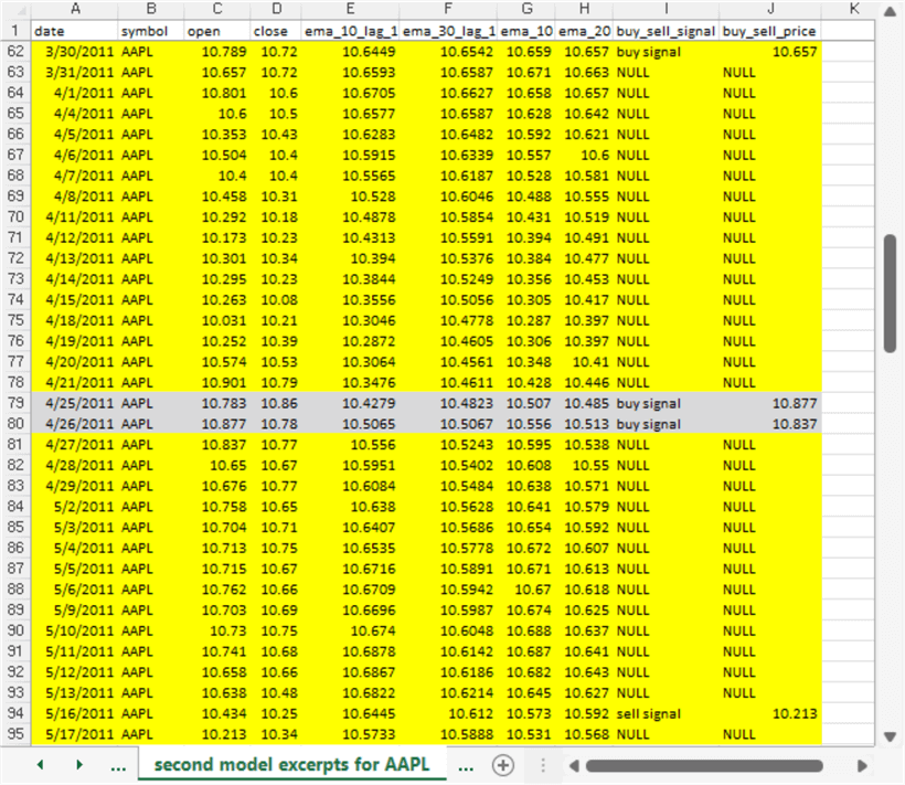
The following screen image shows the log rows associated with the second buy-sell cycle from the second model.

• The buy signal from the second model appears in row 62.
• The buy price appears in the buy_sell_price column of row 62, which references the open column value in row 63. This is because the buy for a security occurs on the first trading day after the buy signal row.
• The sell signal appears in the buy_sell_signal column of row 94, which references the open column value in row 95. Again, this because the signal row for a buy or sell is executed on the first trading day after the signal row.
• The sell price appears in the buy_sell_price column of row 94, which references the open column value in row 95. Again, this is because the execution of an action, such as to sell a security, takes place on the first trading day after the signal row for the action.
• The change in price during the second buy-sell cycle is 10.213, the sell price on 5/17/2011, less 10.657, the buy price on 3/31/2011.
• There are 33 trading days from the buy action that begins the buy-sell cycle on 3/31/2011 through the sell action that ends the buy-sell cycle (on 5/17/2011).
• The screen image below contains two rows with gray instead of yellow backgrounds. The rows with gray backgrounds have date column values of 4/25/2011 and 4/26/2011.
  • These rows have buy signal as a string value in in their buy_sell_signal column.
  • The buy signal values are irrelevant because buy signal values in the buy_sell_signal column are ignored unless they are the row denoting the beginning of a buy-sell cycle.
  • The only buy signal row that can begin a buy-sell cycle is the first row with a buy signal value after the sell signal value in the next to the last row of a preceding buy-sell cycle.

The following screen image shows the log rows associated with the third buy-sell cycle from the second model.

• The buy signal from the second model appears in row 106. This is the buy signal for the third buy-sell cycle in the log from the second model.
• The buy price appears in the buy_sell_price column of row 106, which references the open column value in row 107. This is because the buy for a security occurs on the first trading day after the buy signal row.
• The sell signal appears in the buy_sell_signal column of row 108, which references the open column value in row 109. Again, this is because the signal row for a buy or sell is executed on the first trading day after the signal row.
• The sell price appears in the buy_sell_price column of row 108, which references the open column value in row 109. Again, this is because the execution of an action, such as to sell a security, takes place on the first trading day after the signal row for the action.
• The change in price during the third buy-sell cycle is 10.402, the sell price on 6/7/2011, less 10.557, the buy price on 6/3/2011.
• There are 3 trading days from the buy action that begins the buy-sell cycle on 6/3/2011 through the sell action that ends the buy-sell action (on 6/7/2011).
• The screen image below contains one row with a gray background instead of a yellow background. The row with gray background has a date column value of 6/3/2011.
  • This row has a buy signal as a string value in in its buy_sell_signal column.
  • The buy signal value is irrelevant because a buy signal value in the buy_sell_signal column is ignored unless it is in the row denoting the beginning of a buy-sell cycle.
  • The only buy signal row that can begin a buy-sell cycle is the first row with a buy signal value after the sell signal value in the next to the last row of a preceding buy-sell cycle.

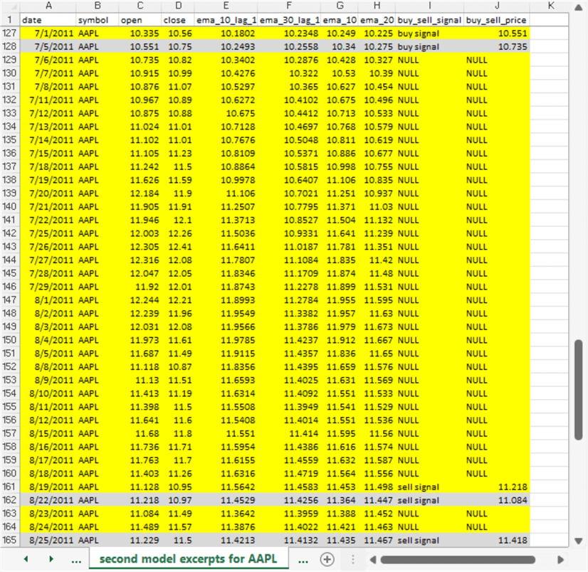
The following screen image shows the log rows associated with the fourth buy-sell cycle from the second model.

• The buy signal for the second model appears in row 127.
• The buy price appears in the buy_sell_price column of row 127, which references the open column value in row 128. This is because the buy action for a security occurs on the first trading day after the buy signal row.
• The sell signal for the buy-sell cycle appears in the buy_sell_signal column of row 161, which references the open column value in row 162. Again, this is because the signal row for a buy or sell recommendation is executed on the first trading day after the signal row.
• The sell price appears in the buy_sell_price column of row 161, which references the open column value in row 162. Again, this is because the execution of a recommendation, such as to sell a security, takes place on the first trading day after the signal row for the recommendation.
• The change in price during the fourth buy-sell cycle is 11.218, the sell price on 8/22/2011, less 10.551, the buy price on 7/5/2011.
• There are 35 trading days from the buy action that begins the buy-sell cycle on 7/5/2011 through the sell action that ends the buy-sell cycle (on 8/22/2011).
• The screen image below contains three rows with gray instead of yellow backgrounds. The rows with gray backgrounds have date column values of 7/5/2011, 8/22/2011 and 8/25/2011.
  • The row with a date value of 7/5/2011 has buy signal as a string value in its buy_sell_signal column. This buy signal value is irrelevant because buy signal values in the buy_sell_signal column are ignored unless they are the row denoting the beginning of a buy-sell cycle. The buy signal for the fourth buy-sell cycle appears in row 127 (on 7/1/2011). The only buy signal row that can begin a buy-sell cycle is the first row with a buy signal value after the sell signal value in the next to the last row of a preceding buy-sell cycle.
  • Rows 162 and 165 each have sell signal values that are irrelevant. This is because neither of these sell signal values follow a buy signal recommendation just before the start of a buy-sell cycle. In fact, the recommendations on rows 162 and 165 follow a preceding sell action that ends a buy-sell cycle. A sell signal recommendation cannot be acted on unless it is tied to a buy signal recommendation.

Sample running balance reports for ticker symbols from AI time series models

The sql script files for each of the two AI time series models in this tip recommend buy and sell dates for a sequence of buy-sell cycles. The scripts in the files also

• Track running balance reports over successive buy-sell cycles from each model
• Count the duration in trading days in successive buy-sell cycles from each model
• Display related information for successive buy-sell cycles from each model
• This summary information is referred to as a buy-sell cycle report.

This section aims to introduce you to contents of buy-sell cycle reports. The source code for generating this information will be reviewed and described in one or more future tips. However, you have the source code for the models in this tip’s download for your own personal study.

The following table presents a pair of screen images for the first and last four buy-sell cycles for the AAPL ticker symbol from the first AI time series model. The information for the first four and last four market cycles appear, respectively, in the top and bottom screen images. Furthermore, the code is copiously commented.

• The summary information for each buy-sell cycle occurs over two rows. The first row is for the buy signal and buy action. Recall the buy signal occurs one day before the buy action.
• The second row for a buy-sell cycle shows the sell signal, sell action, and the performance for the buy-sell cycle.
• Therefore, the information for each buy-sell cycle market report occurs over two rows.

The columns that appear in the screen images below are a subset of those provided by the AI script files.

• The current balance column displays the outcome from an initial investment of $1000 and the gain or loss over successive market cycles of the balance from the preceding market cycle.
  • For example, current balance value on the second row in the top screen image shows that at the end of the first buy-sell cycle, the current balance reflected a gain of 5.70.
    • The percentage point price change per share is 0.57.
    • This percentage price change multiplied by the initial investment of ((1000*.0057) + $1000) results in an ending current balance of $1005.70.
• The buy_sell_cycle_date column shows the first buy-sell cycle
  • begins on 2011-01-06
  • ends on 2011-03-17
• The buy_sell_signal column shows whether each row is for a buy or sell recommendation
  • The buy signal string in row 1 indicates that this row shows buy action information for the first buy-sell cycle.
  • The sell signal string in row 2 indicates that this row shows sell action information for the first buy-sell market cycle.
• The rows in the buy_sell_cycle column show the number of trading days in a buy-sell cycle.
  • For example, there are 49 days in the first buy-sell cycle.
  • This information is useful for assessing the performance of a model that issues buy and sell recommendations for securities over an extended period, such as the 10.5 years of source data as in this tip.
• The current balance column in row 102 within the bottom screen image below displays a final balance after all 51 buy-sell cycles complete. The full buy-sell cycle report contains a buy signal row and a sell signal row for each buy-sell cycle.
  • The final current balance from the first AI time series model is $7,148.81. The percentage change from the initial $1,000 investment before the buy is over 600 percent!
  • This change percentage was achieved over a 10.5 period.

The following table presents a pair of screen images for the first and last four buy-sell cycles for the AAPL ticker symbol from the second AI time series model. This table has the same layout as the preceding table.

• Perhaps the most important point of comparison between the two tables is the current balance for the final trade. In the second pair of screen images below, the final trade results appear on row 58. The current balance after the final trade recommended by the second model is $4,956.09. This compares to value of $7, 148.81 from the first model.
• Because there are 58 rows in the market cycle report below for the second model, there are just 29 trades recommended by the second model versus 51 trades from 102 buy and sell rows recommended by the first model.

Another key take away from the following table for the second model versus the preceding table for the first model is that the models sometimes choose different buy-sell dates over the 10.5 year duration for which the AAPL security is tracked in this tip.

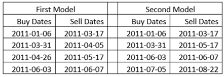
One way to highlight that the buy dates and sell dates across the models are sometimes the same and sometimes different is to list them side by side. The following table lists the first four buy and sell dates from the first model in the first two columns versus the first four buy and sell dates from second model in the second two columns.

• The first pair of buy and sell dates are identical between the two models.
• The second pair of buy and sell dates share the same buy dates, but the sell dates are different between the two models.
• The third pair of buy and sell dates have different buy dates and sell dates between the two models.
• The fourth pair of buy and sell dates have different buy dates and sell dates between the two models. However, the sell date from the first model in the fourth pair matches the sell date from the third pair of buy and sell dates from the second model.

Assessing AI time series model performance

At this point in the tip, you may be wondering which model does best for all or most of the individual ticker symbols and just what exactly does perform better mean. Both models are evaluated with the same set of securities. Therefore, security selection does not affect the evaluation of which does better. Also, comparing the model performance to a broad market index, such as the SPY exchange traded fund, is not necessarily a valid comparison. One or both models could have a smaller return than the SPY just because the S&P 500 index on which the SPY is based, has a changing set of underlying securities over time. Also, both models examined in this tip do not leave their funds invested all the time. This means that the funds are available, at least some of the time, for other purposes, such as investing in more securities, holding in a savings account, or funding special requirements (like going on a lavish vacation). Buying and holding any broad index fund, places those funds at risk all the time. Also, changing the account balance from prior periods (by failing to re-invest gains or losses from prior periods or just withdrawing funds from the account balance) lowers the rate of return.

This tip takes the position that returns generated by each model is a good way of assessing performance. Four different measures of return are evaluated for each model. The prime assessment tool for the model is the comparison of the beginning balance before any trades versus the ending balance after all trades are executed based on model recommendations. This difference captures the performance of the model relative to an arbitrary starting point – namely, the initial account balance before any buy-sell cycles are executed.

• You can represent the difference as the change in dollars from the beginning balance through the ending balance.
• You can also represent the difference as a percentage change from the beginning balance through the ending balance.
• Another way to express the change in account balance within the context of this tip is as a compound annual growth rate over a duration of 10.5 years.
• The last way that this tip assesses model performance is with compound annual growth rate adjusted for days that account balances are at risk.
  • The role of the models used in this tip is to time when to enter and exit trades. Not all trades extend over the same duration.
  • Additionally, there are gaps in trading days from the end of one buy-sell cycle through the beginning of a subsequent buy-sell cycle.
  • The combination of these two issues mean that a balance is not constantly at risk with the models for this tip. Instead, a balance is only at risk during the summed duration of the trades for a security (or a set of securities). Therefore, one thought on how to assess model performance is to adjust the compound annual growth rate over the trading days for which an account balance is at risk.

The following two screen images from Excel workbook files show the outcome from each of the four assessment guidelines for each model on an individual security basis as well as across all six of the securities tracked within this tip. As you can tell from the first row of the worksheet in each image, the first image is for the first model, and the second image is for the second model. The layout of both worksheets is identical, but the returns showing in both workbooks are different. These differences reflect the comparative performance for each model.

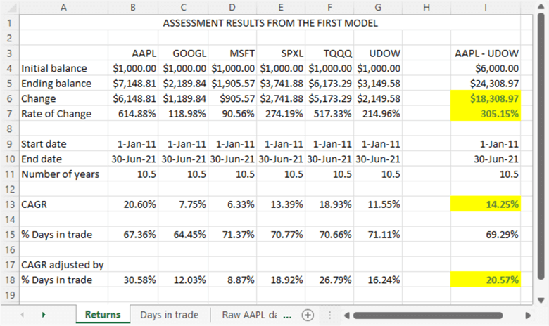
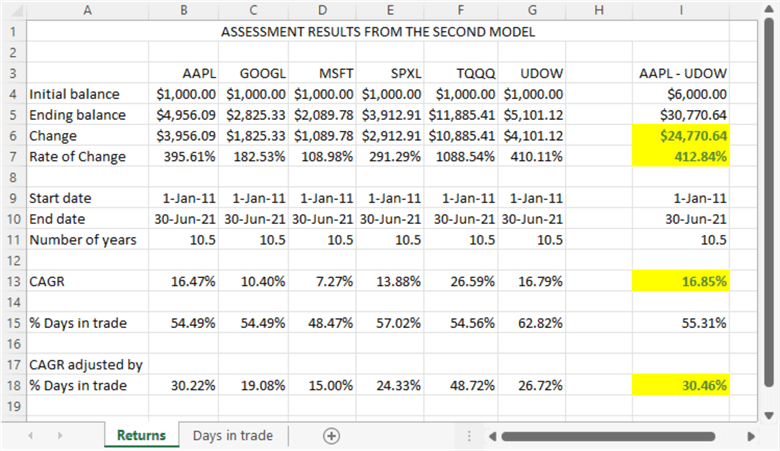
Column I shows aggregate results across the portfolio of all six tickers (AAPL – UDOW). These six securities represent a portfolio of securities. Therefore, it is possible to assess the models based on the portfolio aggregate as well as for each individual security. The four cells that are highlighted with a yellow background in Column I portray the aggregate performance score across all six ticker symbols for each of the four performance metrics.

The aggregate initial balance is $6000, which is the sum of $1000 for each of six tickers; this aggregate is the same for both models. Similarly, the aggregate ending balance is the sum of the ending balance across the six tickers after all recommended trades are completed. The ending balance for the first model is $24,308.97, and the ending balance for the second model is $30,770.64. Therefore, the second model has a substantially greater return over the 10.5 years tracked by this tip.

The change amount represents the ending balance less the initial investment. For the portfolio aggregate of six securities, the first model has a change amount of $18,308.97, and the second model has a change amount of $24,770.64. Therefore, the second model has a substantially greater change over the 10.5 years tracked by this tip.

The first two metrics are assessed in terms of dollars. However, you may care to have a performance metric based on percentage points, such as the rate of change. This approach provides an outcome that is tied not tied to the size of the initial investment. The rate of change is the change amount divided by the initial investment. You can apply the rate of change to any initial investment size and get a return amount that is comparable to the size of the initial investment and the rate of change.

From the worksheet images above, the rate of change for the first model is 305.15% over the 10.5 years tracked by tip, and the rate of change for the second model is 412.84%. Therefore, the second model has a substantially greater rate of change over the 10.5 years tracked by tip.

The compound annual growth rate (CAGR) is the annual percentage per year over a span of years that it takes for an investment to grow from an initial balance to an ending balance. The link for the compound annual growth rate includes an expression for computing the CAGR given an ending balance, an initial balance, and a span of years. This expression is programmed into the two spreadsheets above for the values showing on the thirteenth row.

• The evaluation duration is 10.5 years.
• The initial balance before any trades appears in the fourth row.
• The ending balance after the final trade appears in the fifth row.

The CAGR for the first model is 14.25%. The CAGR for the second model is 16.85%. Therefore, the second model yields superior CAGR value.

The CAGR assumes an investment is at risk for all periods from the initial balance through the ending balance. However, the timing model examined in this tip only puts a current balance at risk for the duration of each set of the buy-sell cycles associated with a ticker symbol. Therefore, current balances are at risk only over the percentage of the total trading dates that are in buy-sell cycles. This percentage appears in the fifteenth row of the two preceding spreadsheets. Row 18 of the spreadsheets above reveals the CAGR adjusted by the percentage of trading dates in buy-sell cycles.

• As you can see, the adjusted CAGR in row 18 is higher for both models than the unadjusted CAGR in row 13. Again, this is because the adjustment accounts for the fact that the models examined in this tip only puts account balances at risk for a fraction of the total trading dates over 10.5 years.
• Row 15 from both of the preceding spreadsheet images shows the percentage of days in trades for the first and second models, respectively. Column I shows that percentage of days in trades over 10.5 years is 69.29% for the first model and only 55.31% for the second model. In other words, the second requires less days in trades to achieve its results.
• Therefore, the second model has a substantially higher CAGR adjusted by % days in trades than the first model. The second model’s advantage is about 10% per year.

Changing the focus from the portfolio aggregate to the individual ticker symbols, a couple of repeatable patterns emerge.

• For five of the six ticker symbols examined in this tip (GOOGL, MSFT, SPXL, TQQQ, and UDOW), the second model generated superior performance. The TQQQ symbol is a standout with a rate of change exceeding 1000% for the second model while other symbols have a rate of change from the second model in the range of around 100% through around 400%
• For the AAPL ticker symbol, the rate of change is much higher for the first model than the second model. In addition, AAPL has a higher rate of change for the first model than any other ticker for the first model.

Next Steps

• This tip is about performance assessment for comparing two AI models programmed in T-SQL. The models illustrate two alternative approaches for implementing the core idea that a downward moving trend of close prices followed by the beginning of upward moving trend of close prices that is a good time to buy a security. The models are different in how far down the downtrend has to go before signaling a downtrend.
• The tip examines four performance metrics to assess which model exhibited better performance. All four metrics assess performance as better the larger the final running balance grows relative to the initial balance before any trades from either model. T-SQL code for implementing each model also computes the running balance over successive trades. A spreadsheet computes the four performance metrics from the list of running balances and other performance indicators for the trades recommended by an AI model.
• The download from this tip includes two sql files one for programming the logic of each model as well as computing metrics on the performance of each buy-sell cycle for each model. Additionally, the download includes an Excel workbook file with two tabs; the sample data for each sql file that implements a model is on a separate tab. Also, the download includes an Excel workbook file with separate tabs for the first two log rows from the first and second models. Finally, the download includes two Excel workbook files with assessment results and expressions for each model.
• Next steps include running the models with the sample data and assessing the performance metrics with the workbook files. Also, you can modify the models as well as the input data to confirm how model design changes and data for different tickers impact model performance.

About the author

Rick Dobson is an author and an individual trader. He is also a SQL Server professional with decades of T-SQL experience that includes authoring books, running a national seminar practice, working for businesses on finance and healthcare development projects, and serving as a regular contributor to MSSQLTips.com. He has been growing his Python skills for more than the past half decade -- especially for data visualization and ETL tasks with JSON and CSV files. His most recent professional passions include financial time series data and analyses, AI models, and statistics. He believes the proper application of these skills can help traders and investors to make more profitable decisions.

This author pledges the content of this article is based on professional experience and not AI generated.

View all my tips