Create and Compare SQL Time Series Models

By: Rick Dobson   |   Updated: 2021-10-07   |   Comments   |   Related: > TSQL

Problem

Demonstrate a framework for creating and comparing time series models with SQL code. Use the models to specify actions to perform now based on reversals in time series trends. Illustrate comparative model performance with multiple different time series.

Solution

Time series data analyses are becoming a significant part of our life as database professionals. Models based on time series offer a powerful tool for projecting recent trends into the future. Over about the past few years from when this article was prepared, it is common to find time series data reports tracking COVID-19 new cases, hospitalizations, and deaths. A decline in the exponential moving average for COVID-19 new cases can result in future declines of COVID-19 hospitalizations and deaths.

This tip compares four time series models that signal when to buy and sell financial securities, such as company stocks or exchange traded funds. A prior tip fully describes how to specify, run, and display results from this type of model with SQL. The models designate when to buy or sell a security based on price trends. For example, when the time series prices for a security starts to decline after a progression of generally rising prices, then it may be profitable to sell the security in order to retain most of the accumulated gains during the time of rising prices.

This tip employs time series price data for financial securities from the Stooq website. One significant advantage of the Stooq website is that it enables the retrieval of price time series for thousands of financial securities in a single step without the need to designate a historical range or a specific symbol for an individual financial security. Beyond that, the data are returned in zipped csv files without the need for any programming. See this prior tip for in-depth coverage of one way to download time series data from the Stooq website to SQL Server.

SQL file code for buy and sell signals as well as buy and sell prices for all symbols

Each of the four models that this tip compares reside in a separate sql file. Within the sql file for a model, the code tracks model outcomes in a log table. The log table for each model preserves a results set for each of three company stocks with symbols of AAPL (for Apple), GOOGL (for Google), and MSFT (for Microsoft) as well as three exchange traded funds with symbols of SPXL, TQQQ, and UDOW. The three exchange traded funds all aim to return three times the daily return of their underlying security, which is the S&P 500 for SPXL, the leading 103 NASDAQ exchange company stocks for TQQQ, and the stocks in the Dow Jones Industrial Average for UDOW.

The following script is an excerpt from the sql file creating a log table with buy and sell signals as well as selected time series values for six stock symbols. There is a separate row in the log table for each trading date and symbol.

• The log from the model for the script below is saved in a SQL Server table named log_for_buy_at_ema_10_gt_20. A case statement for the buy_sell_signal column in the log assigns either a buy signal or a sell signal to each trading date for each symbol.
  • When the exponential moving average with a period length of 10 rises above another exponential moving average with a period length of 20 following one or more periods during which the exponential moving average with a period length of 20 exceeds the exponential moving average with a period length of 10, then a buy signal is assigned.
  • The code for the sell signal Is the inverse of the one for the buy signal. A sell signal is assigned to a row when the exponential moving average with a period length of 20 rises above another exponential moving average with a period length of 10. Again, this condition must hold following a preceding set of one or more rows in which the 10-period exponential moving average was greater than the 20-period exponential moving average.
  • If neither of these two conditions hold for a trading date, then the value in the buy_sell_signal column defaults to a null value.
• A second case statement named buy_sell_price returns buy and sell prices based on whether the buy_signal_signal column has a value of buy signal or sell signal.
  • The buy and sell prices are based on open price values for the row after the buy signal or sell signal. This value is derived with the help of the sql lead function.
  • The reason that buy_sell_price value is derived from the trading date after the buy_sell_signal value is because you cannot assign a buy signal or a sell signal to a row until the trading date closes (the exponential moving average values for buy and sell signals are based on the close prices for a trading date). Therefore, the buy or sell signal is executed on the next trading date. Also, any of the price values (open, high, low, and close) as well as volume of shares exchanged for a trading date are not finalized until after the trading date closes.
• The underlying values for the buy_sell_signal and buy_sell_price are derived from a sub-query named for_buy_sell_log_for_ema_10_vs_20. The sub-query joins two tables:
  • The stooq_prices table with open, high, low, close prices and volumes of shares exchanged on each trading date for a symbol
  • The denormalized_emas table with exponential moving averages for the close prices on each trading date for a symbol
  • The use of a partition by clause in the Windows functions within the for_buy_sell_log_for_ema_10_vs_20 sub-query segments the stooq_prices and denormalized_emas tables by symbol so all the trading dates for GOOGL follow all the trading dates for AAPL.
  • The order by clause within the Windows functions sorts the log rows by trading date within a symbol.
• The output from the following script is a fresh version of the log table.
  • The name of the log table in the following script is log_for_buy_at_ema_10_gt_ema_20. Notice that the log table is named after the criteria for assigning buy signals to rows in the buy_sell_signal column.
  • The log table output for each of the remaining three sql file models is named according to buying and selling criteria for the model implemented by a sql file. The names of these tables are
    • log_for_buy_at_ema_10_gt_30
    • log_for_buy_at_ema_10_gt_50
    • log_for_buy_at_ema_10_gt_30_and_sell_at_10_gt_3
  • The name for the last log table is more elaborate because it uses criteria with different exponential period lengths for assigning buy signals and sell signals.
  • You can learn more about the basics of how to read log files for time series models in this prior tip.

use [DataScience]
go
 
-- create the log for all symbols
drop table if exists dbo.log_for_buy_at_ema_10_gt_20
 
-- create dbo.log_for_buy_at_ema_10_gt_20
select 
 date
,symbol
,[open]
,[close]
,ema_10_lag_1
,ema_20_lag_1
,ema_10
,ema_20
 
-- set buy and sell signals
,case
   when ((ema_10_lag_1 <= ema_20_lag_1) and  (ema_10 > ema_20)) then 'buy signal'
   when ((ema_10_lag_1 >= ema_20_lag_1) and (ema_20 > ema_10)) then 'sell signal'
   else null
 end buy_sell_signal
 
-- set buy and sell prices
,case
   when ((ema_10_lag_1 <= ema_20_lag_1) and  (ema_10 > ema_20)) then open_lead_1
   when ((ema_10_lag_1 >= ema_20_lag_1) and (ema_20 > ema_10)) then open_lead_1
   else null
 end buy_sell_price
 
into dbo.log_for_buy_at_ema_10_gt_20
 
from
(
-- source rows for buy/sell actions
select 
 stooq_prices.* 
,denormalized_emas.ema_10
,denormalized_emas.ema_20
,denormalized_emas.ema_30
,denormalized_emas.ema_50
--,denormalized_emas.ema_200
,lag(denormalized_emas.ema_10,1) over (partition by stooq_prices.symbol 
      order by denormalized_emas.date) ema_10_lag_1
,lag(denormalized_emas.ema_20,1) over (partition by stooq_prices.symbol 
      order by denormalized_emas.date) ema_20_lag_1
,lead(stooq_prices.[open],1) over(partition by stooq_prices.symbol 
      order by  denormalized_emas.date) open_lead_1
 
from DataScience.dbo.stooq_prices
inner join DataScience.dbo.denormalized_emas
on stooq_prices.date = denormalized_emas.date
and stooq_prices.symbol = denormalized_emas.symbol
) for_buy_sell_log_for_ema_10_vs_20

Architecture of SQL code for each symbol

The results set in the log from the previous script for each model is further processed for each of the symbols analyzed in this tip. The main processing steps are highlighted below, and the detailed code is available in the download for this tip. An upcoming tip drills down on the code with step-by-step commentary.

• The first step is to extract from the overall log table for a model, a log table for each security symbol. The order of the symbols as follows.
  • The three company stock symbols (AAPL, GOOGL, and MSFT) are followed by the three exchange traded funds (SPXL, TQQQ, and UDOW).
  • The name of the log table for a specific symbol is symbol_temp_log. This table is freshly re-populated for each successive symbol.
  • The last column in the log table for a symbol is the date for executing a buy signal or a sell signal. Recall that the execution date is one trading date after the assignment of a buy signal or sell signal to a row. The name for this last column in symbol_temp_log is next_date.
  • The symbol_temp_log table has a row for each trading date from the first trading date in 2011 through the last trading date in June of 2021.
• The second step creates and populates a fresh version of the symbol_buy_sell_cycle_date table. This table has two rows for each buy-sell cycle.
  • The first column of the symbol_buy_sell_cycle_date table has a value equal to the symbol currently being processed.
  • The second column has the name buy_sell_cycle_date.
  • Each buy-sell cycle for a symbol has two rows -- one with the date for the buy signal and the other with the date for the sell signal.
  • Depending on the time series data and the model, buy signals and sell signals do not necessarily have to follow one another in an alternating fashion. For example, the initial buy signal for a buy-sell cycle can be followed by one or more other buy signals before a sell signal is issued to close the buy-sell cycle. Similarly, after the sell signal to end a buy-sell cycle, one or more other sell signals may be issued before the next buy signal to start a fresh buy-sell cycle. Therefore, some complimentary rules are needed to pick a unique date for the buy signal and another unique date for the sell signal in each buy-sell cycle. The sql code in the download for each sql model evaluated in this tip reveals how to pick the unique dates for the buy and sell signals in each buy-sell cycle.
  • After designating a buy date and a sell date for each buy-sell cycle in the join of the symbol_temp_log table with the symbol_buy_sell_cycle_date table, you have a data source for evaluating the performance of a model for a symbol. This joined data source is the output from the second step.
• The third step computes two key metrics used to evaluate the performance of a model for a symbol. These key metrics are the percentage price change per buy-sell cycle and the percent of cycles for a symbol having a higher sell price than a buy price. When the sell price for a cycle is higher than the buy price for a cycle, then the cycle is referred to as a winning cycle.
• The first through the third steps are repeated six times in each sql model file -- one for each of the six symbols analyzed and compared in this tip.

Drilling down on percentage price change and percentage winning cycles

The following script excerpt shows how to join selected columns from the symbol_temp_log table with the symbol_buy_sell_cycle_date table as a data source for an outer query. The outer query and an associated Excel workbook file computes the percentage price change per buy-sell cycle and the percent of cycles having a higher sell price than a buy price per model. These actions comprise the second and third processing steps from the itemization of steps in the preceding section. The script excerpt in this section populates the #percent_change_and_percentage_change_per_cycle temp table with the two key performance metrics. Both metrics depend on the price change per cycle for a symbol.

• The script starts by assigning a symbol value, such as AAPL, to the @symbol local variable.

• The percentage change per cycle is computed as the price change for a buy-sell cycle divided by the buy price for the cycle.
• The precent of winning cycles from January 2011 through June 2021 for a symbol within a model is not directly computed within the script excerpt, but its value depends on the number of cycles with a positive price change divided by the total number of buy-sell cycles for a symbol within a model.
• The two metrics are saved in and displayed from the #percent_change_and_percentage_change_per_cycle table. This table contains two rows per cycle – one for the buy price and the other for the sell price of each buy-sell cycle from January 2011 through June 2021.

drop table if exists #percent_change_and_percentage_change_per_cycle
 
-- have to repeat declaration for @symbol in this batch
declare @symbol nvarchar(10) = 'AAPL'
 
select 
    *
   ,case
      when buy_sell_signal = 'sell signal' then
         buy_sell_price
         - (lag([buy_sell_price],1) over(order by buy_sell_cycle_date))  
    end price_change
   ,case
      when buy_sell_signal = 'sell signal' then
         (buy_sell_price
         - (lag([buy_sell_price],1) over(order by buy_sell_cycle_date)))/
         (lag([buy_sell_price],1) over(order by buy_sell_cycle_date))*100
    end percentage_price_change
into #percent_change_and_percentage_change_per_cycle
from
(
-- join of buy_sell_price values from the symbol_temp_log table
-- with buy_sell_cycle_date values from symbol_buy_sell_cycle_date table
-- returns buy and sell prices for each buy_sell cycle
select 
 symbol_temp_log.date
,symbol_temp_log.symbol
,symbol_temp_log.buy_sell_signal
,symbol_temp_log.buy_sell_price
,symbol_temp_log.next_date
,symbol_buy_sell_cycle_date.buy_sell_cycle_date
 
from dbo.symbol_temp_log
inner join dbo.symbol_buy_sell_cycle_date on
symbol_temp_log.next_date = symbol_buy_sell_cycle_date.buy_sell_cycle_date
) buy_sell_prices_for_price_change_per_cycle

The following screen shot is an excerpt from a tab in an Excel workbook with a copied results set for the TQQQ symbol for the model that proposes buy dates on the trading date after the ema_10 value exceeds the ema_20 value. The screen image below displays results for the first five trades.

• The date column shows the buy signal date and the sell signal date for successive buy-sell cycles.
  • For example, cell A2 is the trading date (1/5/2011) before the buy date for the first buy-sell cycle. The actual first buy date (1/6/2011) resides in cell E2. Recall that you cannot know exponential moving averages until after the close of a trading date.
  • The first buy-sell cycle comes to an end on the first trading date after 3/2/2011. This trading date (3/3/2011) is denoted in cell E3.
• Column D displays the buy and sell prices.
  • The buy price for the first buy-sell cycle is 1.6492. This is the open price on 1/6/2011.
  • The sell price is 1.7994, which is the open price on 3/3/2011.
• Column G shows the price change (that is, the sell price less the buy price for a buy-sell cycle).
• Column H shows the percentage price change for a buy-sell cycle.
• Column I contains a value of 1 when the sell price is greater than the buy price and a value of 0 when the sell price is not greater than the buy price.
• Column L shows the value changes of a $1000.00 initial purchase of shares for the symbol over the first five trades.
  • For example, the $1000.00 share purchase at the close of the first buy-sell cycle increased to a value of $1091.00.
  • The second cycle reduced the account balance for the TQQQ symbol from $1091.00 to $1030.89 because the second cycle had a percentage_price_change value of -5.51 percent.
  • The details of how to compute the balance at the end of the fifth cycle appear below.
    • This balance change from the preceding buy-sell cycle was driven by the -10.79 percent price change for the fifth buy-sell cycle applied to the ending balance of $885.00 for the fourth trade.
    • The balance at the end of the fifth buy-sell cycle falls to $789.51.
• As you can see, the balances are cumulative in the sense that the ending balance from the preceding buy-sell cycle is the reference value for the beginning balance of the current buy-sell cycle.

The next screen shot shows the final five trades for the TQQQ symbol for the model that specifies a buy when the ema_10 value exceeds the ema_20 value.

• Although just one of the first five trades was a winning trade, the last five trades were winning ones in four of five instances.
• One especially interesting data point in the screen shot below appears in cell H113. This cell reports the percentage price change as 99.02. It is for the first buy-sell cycle after the COVID-19 crash beginning in late February through early April in 2020. As you can see,
  • The buy-sell cycle starts on April 16, 2020
  • The buy-sell cycle ends on September 14, 2020.
• Also, the value in cell L113 shows the ending balance at the close of the first buy-sell cycle after the COVID-19 crash growing to $5930.97.
  • This outcome is about $2950 greater than the prior ending balance.
  • The prior trade ended on February 27, 2020 – towards the very beginning of the COVID-19 crash.
• As a result of the overall ratio of winning cycles to total cycles for all the trades from January 2011 through June 2021, the percent of winning cycles is 40.68.
  • Therefore, the percent of non-winning cycles is 59.32.
  • Even with a non-winning cycle percentage of over 59 percent, the model was able to pick buy and sell dates so the balance for the TQQQ security grew from $1000 to more than $6173 in just 59 trades.

A snapshot of a rally buy-sell cycle

The following screen shot shows a chart for a rally from mid-April 2020 through early-November 2020 buy-sell cycle for the security with a ticker symbol of AAPL. This is an example of a winning cycle for the model that assigns buy and sell signals based on ten-period and fifty-period exponential moving averages. As the chart shows, prices can go up and down throughout a cycle. Because this cycle is for the rally starting after the COVID-19 crash, the prices rise during most of this very long buy-sell cycle. The rally buy-sell cycle in the image below is defined by the cross-over dates for the ten-period ema and the fifty-period ema.

• You can observe a green line (ema_10) in the image below crossing from below to above a red line (ema_50). This event marks the buy date for the cycle.
• The beginning cross-over occurs after the green line craters from the COVID-19 crash and confirms the beginning of a recovery by showing the cross-over of the green line above the red line.
• The close of the buy-sell cycle occurs on the day after a cross-over of the green line below the red line.

Overall Performance comparisons for symbols across four models

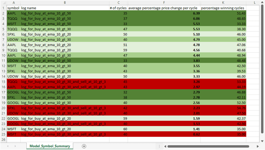
Another way of examining performance differences is by model comparisons. The log name column in the screen shot below has 24 data rows – six rows each for each of the four models examined in this tip. The rows are sorted by the order of their average percentage price change per cycle value; the font for this column is bold. The last column denotes the percentage of winning cycles for the model on that row; rows are not sorted by this column value.

Each of the six rows for each of the four models is for a symbol – namely, AAPL, GOOGL, MSFT, SPXL, TQQQ, and UDOW. The symbol names appear in column A. A row’s background color denotes the type of model for that row in the summary table.

• Dark green is for the model that buys when ema_10 rises above ema_50
• An intermediate shade of green is for the model that buys when ema_10_rises above ema_30
• The lightest shade of green is for the model that buys when ema_10_rises above ema_20
• Red is for the model that buys when ema_10 rises above ema_30 and sells when ema_10 rises above ema_3

The closer the color for a model is towards the top of the summary table, the better performance of that model for a symbol based on average percentage price change per cycle.

• The model that buys when ema_10 rises above ema_50 delivers the best performance. Four of its six rows are in the top half of the following table, and none of its rows are among the bottom six rows in the table.
• The model that buys when ema_10 rises above ema_30 and sells when ema_10 rises above ema_3 delivers the worst performance. Four of its rows are in the bottom six rows of the following table, and all six of its rows are in the bottom half of the table.
• The remaining two models deliver intermediate levels of performance between the best and worst performing models.

A note about the source data for security prices examined in this tip

Stooq data are very close to, but not identical to, Yahoo Finance data. While Yahoo Finance data is a traditional favorite source for trading analysts, Stooq data has some distinct advantages. This section briefly points to some of the most significant similarities and differences of the two alternative data sources for security prices. The focus is on open prices because the models within this tip project buy and sell prices based on open prices.

The following screen shot illustrates the exceedingly close overlap between Yahoo Finance and Stooq open prices for the SPXL symbol. The data are for all trading dates from the beginning of January 2011 through the end of June 2021. Here are key points to ponder.

• The coefficient of determination (R²) is .9998. Therefore, the variance of the Stooq open prices is almost completely accounted for by the variance of Yahoo Finance open prices.
• Additionally, the equation for predicting Stooq open prices from the Yahoo Finance open prices has a slope that is nearly one with an x-intercept that is very close to zero. This points to the fact that the Stooq open prices are nearly identical to the Yahoo Finance open prices.

To better understand the points of divergence between Yahoo Finance and Stooq open prices, separate regressions were run predicting Stooq open prices from Yahoo Finance open prices. The chart on the left is for the first month of data (January 2011). The chart on the right is for the last month of data (June 2021). As you can see, there is no divergence in the last month (100 percent of the variance of the Stooq open prices is accounted for by the Yahoo Finance open prices). Also, there is only a very slight divergence in the first month (99.94 percent of the variance of the Stooq open prices is accounted for by the variance of the Yahoo Finance open prices).

Finally, I scanned on a side-by-side basis across all periods from the first through the last month. This scan revealed the gradual complete convergence of Stooq open prices with Yahoo Finance open prices from the first through the last month.

If Stooq prices are not identical to Yahoo Finance prices, why bother with Stooq open prices?

• As indicated above, the differences are not sufficiently great to miss identifying trends with either source of data.
• Second, Stooq allows you to download all its US market data without the need for designating for which specific symbols you seek data or over which historical periods you want data.
• Third, Stooq offers the download of historical security prices for non-US markets with the same kind of ease. I notice links within the Stooq website for the download of historical market data from the UK, Japan, Hong Kong, Germany, Poland, and Hungary.

Next Steps

This tip shows a framework for comparing time series models with results sets from SQL code passed to an Excel workbook file. The models are about designating decisions, such as to buy or to sell a security based on exponential moving averages for time series values. The models capture a reversal in time series values and presumes the reversed direction of two moving averages will continue until the moving averages suggest another reversal of direction started.

The comparative results reported in this tip suggest relatively better performance for some models and some security symbols. Additional data mining and modeling refinement with more symbols is required to confirm the robustness of the time series models. The purpose of the models studied in this tip is to make a prediction about when to make a decision based on some time series values. In order to evaluate predictions, it is common to use techniques such as cross validation as well as comparing results for a training set of data versus a hold-out sample for a different set of data points. It is my plan to apply these model validation techniques in the future, but I also encourage you to try them on your own even before a future tip appears on model validation techniques.

In the meantime, you may be interested in the support files for this tip, which are available in the download for this file. These include:

• Four sql files – one for each model
• Two csv files with data for stooq_prices and denormalized_emas tables
• A comparison Excel workbook file with data for all symbols on separate tabs for the buy_at_ema_10_gt_20 model
• A comparison Excel workbook file with average percentage price change per cycle and percentage winning cycles for 24 model-symbol combinations
• A comparison Excel workbook file for comparing Stooq open prices with Yahoo Finance open prices

About the author

Rick Dobson is an author and an individual trader. He is also a SQL Server professional with decades of T-SQL experience that includes authoring books, running a national seminar practice, working for businesses on finance and healthcare development projects, and serving as a regular contributor to MSSQLTips.com. He has been growing his Python skills for more than the past half decade -- especially for data visualization and ETL tasks with JSON and CSV files. His most recent professional passions include financial time series data and analyses, AI models, and statistics. He believes the proper application of these skills can help traders and investors to make more profitable decisions.

This author pledges the content of this article is based on professional experience and not AI generated.

View all my tips