Problem
I need a way of detecting reversals for time series data within SQL Server. I heard the Relative Strength Index can serve as an indicator of reversals in time series. Please show me how to compute this indicator with T-SQL. Also, indicate ways to make the computations relatively easy to perform for different time series over different date ranges for time series data in SQL Server.
Solution
A reversal in a time series signals a turn-around in the direction of the values within a time series. It is often useful to learn about reversals as quickly as possible so your business can avoid bad consequences from unexpected outcomes. For example, it is better to have an ample supply of materials in inventory for servicing orders before clients make other arrangements for meeting their requirements because of unshipped orders from your firm. Reversal detection is an especially popular topic for financial securities time series. You can sometimes achieve more gain from a security by purchasing stock in a company before others buy it and drive the price up. Similarly, you can minimize the loss from a security’s price through by selling it in the initial stages of a price decline.
There are multiple indicators for shining a light on time series reversals. One indicator that has stood the test of time is the Relative Strength Index (RSI). This indicator was initially proposed back in 1978 by J. Welles Wilder in a book titled “New Concepts in Technical Trading Systems”. Numerous authors contributed content about how to compute and/or use RSI (here, here, here, and here). It is the continuing stream of the content about RSI over a span of decades which suggests its value for trend reversal detection.
A prior MSSQLTips.com article from several years ago illustrated how to compute the indicator with a T-SQL script as well as demonstrate a use case for the RSI. This tip revisits the topic to describe in detail an algorithm for computing RSI values. The description is then linked to T-SQL code so that you can clearly understand how different code blocks link to elements in the RSI computational algorithm. The earlier T-SQL code for computing RSI is improved to have more precision and to be more flexible in accommodating different ticker symbols and different date ranges. Beyond these refinements, this tip illustrates how to compute RSI values for time series from the Stooq.com historical data source, which is free and easy to use with SQL Server.
RSI computational algorithm
The RSI is an oscillator. That is, its range of values extend from a high value of 100 through a low value of 0. RSI values depend on the ratio of the average percentage gain to the average percentage loss over a set of periods within a timeframe. The default timeframe value of 14 trading days is widely used, but some analysts prefer longer or shorter timeframes. Other analysts apply the RSI with multiple timeframes to facilitate their analyses of reversals in time series. This tip focuses on how to compute the RSI with its default value of 14 periods. The tip also focuses on the computation and verification of RSI values for three securities.
The RSI is computed based on changes in some criterion value, such as close prices, from one period to the next within its timeframe. When the price rises from one period to the next one, this is a gain. When the price falls from one period to the next one, this is a loss. Losses are represented as positive values so gains and losses can be compared to each other. There are two different methods used for computing the average gain and the average loss.
- A simple arithmetic average is the first method. This method is applied to compute the average percentage gain and average percentage loss over the initial periods within the first timeframe instance. With the default value of 14 periods for a timeframe, the RSI for the fifteenth period depends indirectly on the ratio of the average gain to the average loss over the first fourteen periods. Prior to the fifteenth period, there are no RSI values.
- For all subsequent time periods, average gain and average loss are computed as a weighted average of the prior period’s percentage gain or loss and the current period’s percentage gain or loss. When using a timeframe of 14 periods, the expressions for average gain and average loss in the subsequent periods are as follows.
Average gain = ((previous period average gain) X 13) + (current period gain))/14
Average loss = ((previous period average loss) X 13) + (current period loss))/14
The next two steps are the computation of the RS and the RSI. The RSI depends on the RS, and the RS is computed as the ratio of the average gain to the average loss for the current period. This assesses how well gains are doing relative to losses over a timeframe of periods ending in the current period. Therefore, the expression for RS in the current period is
RS = (Average gain in current period)/(Average loss in current period)
If the average loss equals 0 because the all the previous periods returned gains, then the prior RS expression does not compute because of a 0 divisor. In such a situation, RS should be assigned a value of 0.
The RSI is computed with the following expression. It is this expression which causes the RSI to vary between 0 and 100.
RSI = 100 – (100/(1 + RS))
In practice, RSI rarely reaches its theoretical extreme values of 0 and 100. If RS equals 0 because all the periods in the timeframe have a 0 loss, then RSI equates to 0. As the average loss for a period grows from 0 in comparison to the average gain, RSI increases in value relative to its theoretical limit of 100.
Two RSI use cases
As RSI values change direction from approaching a very high value to approaching a very low value, the RSI indicates a reversal from a high average gain towards approaching a low average percentage gain. Conversely, decreasing RSI values towards a very low value, sometimes called an oversold price, and back in the direction of very high RSI values, sometimes called overbought prices, mark a reversal from low or declining prices towards increasing prices.
The centerline RSI values of around 50 are also sometimes used in reversal analyses.
- When RSI initially rises from oversold prices towards the centerline, but then fails to pierce the centerline value or even a value in between the centerline value and an oversold RSI value, then a trader can be warned to not buy the security because continued gains are not likely.
- Conversely, when RSI falls from overbought levels towards the centerline, but then reverses in the direction of overbought RSI levels, then a trader can keep holding the security in order to receive more gains from a trade.
The sample dataset for this tip
The sample dataset for this tip includes selected time series data for three ticker symbols from the stooq_prices table in the DataScience database. Three csv files are included in the download for this tip with the time series data for which RSI values are computed. Stooq.com maintains a free historical database for stock prices. A prior tip introduces SQL Server professionals to this data source.
The query below followed by its results set selects the three ticker symbols for which RSI values are computed in this tip.
-- ticker symbols referenced in tip
select distinct symbol
from [DataScience].[dbo].[stooq_prices]
where symbol in ('AAPL', 'GOOGL', 'MSFT')

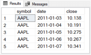
The next query and its results set shows the first five time series records for the AAPL ticker that are included in this tip.
-- display initial 5 time series rows for AAPL
select top 5 symbol, date, [close]
from [DataScience].[dbo].[stooq_prices]
where symbol = 'AAPL'
order by symbol, date asc
The following query and results set display the last five records for the GOOGL ticker that are included in this tip.
-- display most recent 5 time series rows for GOOGL
drop table if exists #most_reent_from_GOOGL

select top 5 symbol, date, [close]
into #most_reent_from_GOOGL
from [DataScience].[dbo].[stooq_prices]
where symbol = 'GOOGL'
order by symbol, date desc

select *
from #most_reent_from_GOOGL
order by date

The query below generates a results set with 82 rows for the 82 trading dates from 2021-01-01 through 2021-04-30. The two following excerpts from the results set show, respectively, the first and last ten trading dates from the results set. Notice the @start_date specifies January 1, 2021 as the start date and April 30, 2021 as the end date.
-- display time series rows for MSFT
-- from 2021-01-01 through 2021-06-3011
declare
 @symbol varchar(5) = 'MSFT'
,@start_date date = '2021-01-01'
,@end_date date = '2021-04-30'

select symbol, date, [close]
from [DataScience].[dbo].[stooq_prices]
where symbol = @symbol
and date >= @start_date and date <= @end_date
Here is an excerpt with the first ten rows from the results set for the preceding query. Notice the first trading date is not until January 4, 2021. Because Friday January 1, 2021 is a stock market holiday and January 2 and 3 are weekend days during which the stock market is closed, the first trading date is not until January 4, 2021. January 9 and 10 are weekend dates. Therefore, these dates are also missing from the time series.

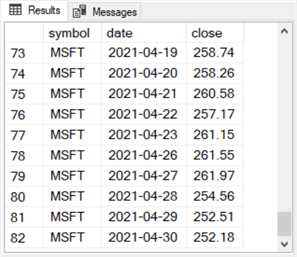
Here is an excerpt with the last ten rows from the results set for the preceding query. The row numbers are 73 through 82. The last row number is 82 because there 82 trading dates in the date range for this tip. The calendar dates April 24, 2021 and April 25, 2021 are weekend days on which the US stock market is closed. Therefore, these two weekend dates do not appear in the time series.
Here are three more queries that show the count of trading dates in this tip for each of the three ticker symbols in the tip. These queries reference three local variable (@symbol, @start_date, and @end_date) from the top of the preceding query.
-- display count of MSFT time series dates in date range
set @symbol = 'MSFT'
select count(date) [count of MSFT dates in date range]
from [DataScience].[dbo].[stooq_prices]
where symbol = @symbol
and date >= @start_date and date <= @end_date


-- display count of GOOGL time series dates in date range
set @symbol = 'GOOGL'
select count(date) [count of GOOGL dates in date range]
from [DataScience].[dbo].[stooq_prices]
where symbol = @symbol
and date >= @start_date and date <= @end_date

-- display count of AAPL time series dates in date range
set @symbol = 'AAPL'
select count(date) [count of AAPL dates in date range]
from [DataScience].[dbo].[stooq_prices]
where symbol = @symbol
and date >= @start_date and date <= @end_date
Here’s the results sets from the three select statements in the preceding code excerpt. This query confirms that each ticker symbol in the dataset for this tip has data for 82 trading dates.

T-SQL script for computing RSI values based on a time series of 82 rows
There are two main parts to the T-SQL code for computing RSI values. The first part creates a temp table and populates selected column values in the table of 82 rows. The second part focuses on computing RSI column values for the temp table initialized in the first part. In addition, the second part also populates selected other columns, such as for average gain and average loss, which are required to compute RSI values.
Initializing a temp table with a time series values for computing RSI values
The script for the first part appears in the code excerpt listed below. A use statement for the DataScience commences the script. The use statement is followed by a declare statement for three local variables named @symbol, @start_date, and @end_date. By changing the values assigned to the local variables, you can re-specify the ticker symbol as well as the start and end dates for which RSI values are computed.
The script excerpt includes an outer query and an inner query. The inner query pulls time series data for the outer query. The outer query initializes and populates with an into clause a temp table named #for_all_avg_gain_loss.
The inner query named for_14_row_avg_gain_loss pulls data from a table named stooq_prices in the DataScience database. The stooq_prices table is queried in the preceding section to familiarize you with some types of data it contains. The columns extracted with the inner query include symbol, date, and close. Additionally, several computed fields are populated in the subquery and further modified in the outer query as well as some trailing T-SQL code.
- The row_number field makes it easy to reference rows based on date. Row order matters when computing RSI values.
- The change, gain, and loss fields are derived either directly or indirectly from the close field. The change field is the current row’s close value less the preceding row’s close value. This definition allows for the change field’s value to be positive, negative, zero, or null.
- The change field is positive when the close value in the current row is greater than close value in the preceding row.
- The change field is negative when close in the current row is less than the close value in the preceding row.
- The change field equals zero when the close values in the current and preceding rows equal one another.
- The change field is null for the first row because there is no preceding row for the first row. The code in the script below transforms null values to 0 with an isnull() function.
- When the change field is positive for a row then
- its value is assigned to the gain column
- and 0 is assigned to the loss column
- When the change field is negative for a row then
- its absolute function value is assigned to the loss column
- and 0 is assigned to the gain column
- When the change field is 0 for a row then both the gain and loss column values are assigned a value of 0.
- When the change field is null for a row then the gain and loss column values are assigned a value of 0.
- The gain and loss columns are inputs to arithmetic average functions for the first fourteen rows in the temp table.
- The arithmetic average function values are assigned to the avg_gain and avg_loss columns in the fourteenth row of the temp table.
- For other rows in the temp table, null values are assigned to the avg_gain and avg_loss columns.
The outer query computes average gain and average loss values over the first fourteen rows of the #for_all_avg_gain_loss table. The outer query also specifies two columns named “relative strength (rs)” and rsi for the #for_all_avg_gain_loss table. These columns are for storing RS and RSI column values computed in the second part of the T-SQL code. At this point in the process, the values for these two columns are specified to contain null values.
After the initial select statement with inner and outer queries, a pair of update statements moves the avg_gain and avg_loss values from the fourteenth row to the fifteenth row and clears the avg_gain and avg_loss values from the fourteenth row. This movement of two column values from the fourteenth to the fifteenth row is necessary because the average of the first fourteen rows in the gain and loss columns is computed with a SQL Server avg window function. The preceding and current row clause of the function computes the average gain or loss and stores the average in the current row (row 14). However, the RSI computational algorithm calls for the first average gain and loss column values being saved in the following row (row 15 with the default timeframe of 14 periods).
The final statement in the script below is a select statement that displays the contents of the #for_all_avg_gain_loss table.
use DataScience
go


-- can respecify @symbol, @start_date, and @end_date
-- to modify the data pulled from a database of time series
declare
 @symbol varchar(5) = 'GOOGL'
,@start_date date = '2021-01-01'
,@end_date date = '2021-04-30'

-- create #for_all_avg_gain_loss
-- populate row 14 for avg_gain and avg_loss
-- then move avg_gain and avg_loss to row 15

drop table if exists #for_all_avg_gain_loss

-- for avg_gain and avg_loss for row 15
-- and base table for updating
select
row_number() over (order by date) row_number
,symbol
,[date]
,[close]
,round(isnull([close]
 - lag([close],1) over (order by date),0),5) change
,round(isnull(gain,0),5) gain
,round(isnull(abs(loss),0),5) loss
,
round(
case
 when row_number <= 13 then null
 when row_number = 14 then
  avg(round(isnull(gain,0),5)) over
  (order by [date] rows between 13 preceding and current row)
end
,5) avg_gain
,
round(
case
 when row_number <= 13 then null
 when row_number = 14 then
  avg(round(isnull(abs(loss),0),5)) over
  (order by [date] rows between 13 preceding and current row)
end
,5) avg_loss
,cast(NULL as real) [relative strength (rs)]
,cast(NULL as real) [rsi]
into #for_all_avg_gain_loss
from
(
-- for gains and losses
select
symbol
,[date]
,row_number() over (order by [date]) row_number
,[close]
,[close]-(lag([close]) over(order by date)) change
,
case
when ([close]-(lag([close]) over(order by date))) > 0
 then [close]-(lag([close]) over(order by date))
when ([close]-(lag([close]) over(order by date))) = 0
 then 0
end gain
,
case
when ([close]-(lag([close]) over(order by date))) < 0
 then [close]-(lag([close]) over(order by date))
when ([close]-(lag([close]) over(order by date))) = 0
 then 0
end loss
from dbo.stooq_prices
where symbol = @symbol and date >= @start_date and date <= @end_date
) for_14_row_avg_gain_loss

-- move avg_gain and avg_loss for row_number 14
-- to avg_gain and avg_loss for row_number 15
-- and assign null values to avg_gain and avg_loss for row_number 14
update #for_all_avg_gain_loss
set avg_gain = (select avg_gain  from #for_all_avg_gain_loss where row_number = 14),
    avg_loss = (select avg_loss  from #for_all_avg_gain_loss where row_number = 14)
where row_number = 15
update #for_all_avg_gain_loss
set avg_gain = null,
    avg_loss = null
where row_number = 14

-- basic data and computation of first 14 rows
select * from #for_all_avg_gain_loss
Here are two excerpts from the results set for the select statement at the end of the preceding script.
- The first excerpt is for the first fifteen rows.
- The symbol, date, and close column values are extracted from stooq_prices.
- The row_number column values are derived from a row_number() function.
- The change, gain, and loss column values are based on expressions from inner and outer queries for close column values.
- The avg_gain and avg_loss column values for the fifteenth row are based, respectively, on the arithmetic average of the gain and loss column values over the first fourteen rows of the #for_all_avg_gain_loss table. These values are derived through a SQL Server avg window function and a couple of update statements that copy the computed values from row fourteen to row fifteen.
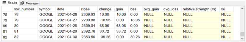
- The second excerpt is for the last five rows in the #for_all_avg_gain_loss table.
- The very last row has a row_number value of 82 because there are 82 rows of source data per time series within this tip. Each ticker symbol corresponds to a distinct time series.
- The avg_gain and avg_loss columns in these last five rows have null values because they require expressions implemented in the second part of the T-SQL code for RSI values.
- Critically, the “relative strength (rs)” and rsi columns also have null values in this excerpt and the preceding one. The code for computing these column values is presented and discussed in the next sub-section.

Computing RS and RSI as well as avg_gain and avg_loss for rows after row 15 in #for_all_avg_gain_loss
After the 15th row, avg_gain and avg_loss column values depend on the weighted average of two rows instead of the arithmetic average of the preceding 14 rows. For example, the avg_loss column value for the 16th row depends on the weighted average of the avg_loss column value for the 15th row and loss column value for the 16th row. Because RS column values depend on avg_gain and avg_loss values from the current and the prior rows and RSI column values depend on RS column values, each row after the 15th row depends on column values from two rows. For these reasons, it is necessary to compute the RS and RSI column values in a loop where each pass through the loop processes values from two rows.
The following script shows the T-SQL for implementing this kind of dependence on two rows for avg_gain and avg_loss column values. The script is heavily commented for details so that this tip’s code commentary focuses just on major issues.
- The script starts with a sequence of local variable declarations to help computing avg_gain, avg_loss, RS and RSI column values. In addition, the @row_number local variable is initialized to 15. The @row_number local variable assists in managing passage through a while loop controlling access to successive pairs of rows, such as (15 and 16), (16 and 17), and (17 and 18).
- After the variable declarations, a while loop uses the @row_number local variable to control access to a succession of row pairs in the #for_all_avg_gain_loss temp table. The first pair or rows accessed is 15 and 16, and the last pair of rows accessed is 81 and 82. Recall that the last row of data in this RSI computation demonstration is row 82.
- Within the while loop, the prior row refers to the first member of each pair, and the current row refers to the second member of each pair.
- Therefore, on the first pass through the loop, the prior row is for row 15 and the current row is for row 16.
- On the final pass through the loop, the prior row is for row 81 and the current row is for row 82.
- Each pass through the loop invokes two update statements. The first update statement is for the prior row, and the second update statement is for the current row.
- The final select statement in the script below displays the computed RS and RSI values in the script below.
-- declare local variables for Relative Strength
-- and Relative Strength Index (rsi) computation
declare @date_cnt int = (select count(date) from #for_all_avg_gain_loss)
,@row_number int = 15
,@gain_prior money
,@loss_prior money
,@avg_gain_prior money
,@avg_loss_prior money
,@gain_current money
,@loss_current money
,@avg_gain_current money
,@avg_loss_current money
,@rs_prior real
,@rsi_prior real
,@rs_current real
,@rsi_current real

---------------------------------------------------------------------------

-- start looping through rows after 14th row until last row
-- process rows iteratively two at a time
while @row_number > 14 and @row_number <=
 (select count(date) from #for_all_avg_gain_loss)
begin


-- assign values to local variables for prior and current rows
-- initially 15 denotes prior row and 16 denotes current row
-- pairs of rows are successively (15,16), (16,17), (17,18)...
select
 @gain_prior = isnull((select gain from #for_all_avg_gain_loss
    where row_number = @row_number),0)
,@loss_prior = abs(isnull((select loss from #for_all_avg_gain_loss
    where row_number = @row_number),0))
,@avg_gain_prior = (select avg_gain from #for_all_avg_gain_loss
    where row_number = @row_number)
,@avg_loss_prior  = abs((select avg_loss from #for_all_avg_gain_loss
    where row_number = @row_number))
,@gain_current = isnull((select gain from #for_all_avg_gain_loss
    where row_number = @row_number + 1),0)
,@loss_current = abs(isnull((select loss from #for_all_avg_gain_loss
    where row_number = @row_number + 1),0))
,@avg_gain_current = (@avg_gain_prior*13 + @gain_current)/14
,@avg_loss_current = (@avg_loss_prior*13 + @loss_current)/14


-- update prior row
update #for_all_avg_gain_loss
set
 [relative strength (rs)] = @avg_gain_prior/@avg_loss_prior
 ,rsi =
  case
  when @avg_loss_prior != 0 then
  (100 - (100/(1+(@avg_gain_prior/@avg_loss_prior))))
  else
  100
  end
where #for_all_avg_gain_loss.row_number = @row_number

-- update current row
update #for_all_avg_gain_loss
set
  avg_gain = ((@avg_gain_prior*13) + @gain_current)/14
 ,avg_loss = ((@avg_loss_prior*13) + @loss_current)/14
 ,[relative strength (rs)] =
  (((@avg_gain_prior*13) + @gain_current)/14)
  /(((@avg_loss_prior*13) + @loss_current)/14)
 ,rsi =
  case
  when @avg_loss_current != 0 then
  (100 - (100/(1+(@avg_gain_current/@avg_loss_current))))
  else
  100
  end
where #for_all_avg_gain_loss.row_number = @row_number+1

-- increment @row_number by 1 to get to
-- the next two rows to process for rsi
set @row_number = @row_number + 1

end


-- for display of computed RS and RSI values
-- as well as comparison of RSI from T-SQL
-- code to RSI from Excel
select *
from #for_all_avg_gain_loss
where row_number >= 15
order by date
Here are two excerpts from the results set for the select statement at the end of the preceding script.
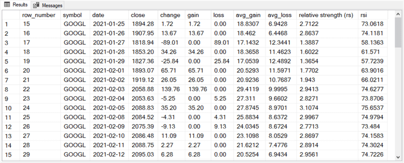
- The first results set excerpt displays RS and RSI values along with other column values that contribute directly or indirectly to RS and RSI values.
- These results are for rows with row_number values of 15 through 29.
- Recall that the algorithm used for computing RSI values does not generate results until the fifteenth row.
- You can also compare the row with a row_number value of 15 in this subsection to the row with the same row_number value from the first results set in the prior subsection. As you can see, the values are the same in both results set excerpts with the exception of the RS and RSI columns. The code for the prior subsection did not compute values for these two columns.
- The second results set excerpt displays the final five rows from the preceding script.
- The date column value for the last row in this excerpt is 2021-04-30, which is for the final row in the source data.
- Also, the close column values match exactly in this results set excerpt versus the second results set excerpt in the prior subsection.
- Of course, the most important feature of the second results set excerpt below is that it has numeric RS and RSI column values. The second results set excerpt from the prior subsection has null values in its RS and RSI columns. Furthermore, the RS and RSI column values correspond to the values generated for these indicators by their equations in the “RSI computational algorithm” section.

Validating T-SQL code for RSI values
This final tip section aims to validate the T-SQL code for computing RSI values by comparing results from the T-SQL code from this tip with another source based on a spreadsheet. The spreadsheet was published along with a technical trading tip from StockCharts.com. The results are compared for three ticker symbols (AAPL, GOOGL, MSFT) for trading dates from January 4, 2021 through April 30, 2021. Close prices are derived from the Stooq.com database. If you change any of these conditions, you can obtain different results.
- For example, iterative algorithms for technical indicators like RSI and exponential moving averages will return different results for different amounts of historical data.
- Stooq.com prices do not exactly match Yahoo Finance historical stock prices for all symbols for all trading dates. This is likely true for other historical stock price data sources.
- Finally, spreadsheets and SQL databases can represent the same underlying stock price with different degrees of precision and rounding. For this reason, very close to a perfect match is as good as you can expect for this kind of work.
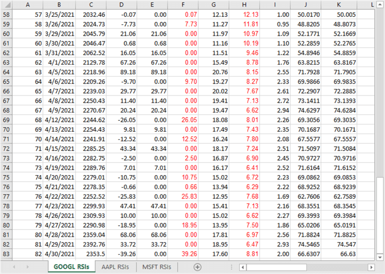
The following two screen shots show the first and last 26 rows of the GOOGL RSIs tab in the “RSI workbook for GOOGL and AAPL and MSFT.xlsx” file.
- Column C contains close price values for the date values in column B.
- Columns D through H show values, but the cells in these columns contain expressions to support the computation of RSI indicator values based on a timeframe of 14 periods.
- Columns I and J compute RS and RSI indicator values based on preceding columns in spreadsheet.
- Column K displays RSI values calculated from the T-SQL in the preceding section.

Here is an image of a scattergram of the RSI values from the T-SQL scripts in the preceding section versus the RSI values from the spreadsheet. The slope, intercept, and R2 for a trend line through the scattergram points appear in the spreadsheet chart.
- The R2 value is 1. This means all the variance from the T-SQL RSI values is accounted for by the Excel RSI values. In other words, the line through the scattergram points is a perfect fit.
- The slope and x intercept for the trend line are, respectively, 0.9997 and 0.0128. These values reflect a nearly perfect fit of the line through the points.

The following table shows the trend line statistics for each of the three symbols. The main point of this table is that for all three symbols the variance of the T-SQL RSI values is completely accounted for by the variance of Excel workbook file (because R2 = 1). The T-SQL presented in this tip matches the corresponding results from the spreadsheet file available from the StockCharts.com site as well as from download for this tip.

Next Steps
RSI is a powerful tool for detecting reversals in time series data. Different stock technical analysts and traders use RSI in different ways to detect reversals in time series, such as daily close prices for a stock. Reversals are useful with stock time series because they may point to times when it might be profitable to buy and sell a security at a profit. You can learn more about how RSI values are used to detect reversals in this prior MSSQLTips.com tip as well as these other Internet resources (here, here, here, and here).
Your next steps with this tip are to confirm that you can detect reversals for any financial security ticker over whatever date ranges you prefer to analyze. By examining how RSI reversal detection worked in the past for identifying profitable trades, you can discover how it may work in the future.
The download for this tip includes three files that will allow you to replicate the results prepared in this tip. The download includes:
- Two T-SQL script files – one for computing RSI values and another for queries with the raw time series data in this tip
- Three csv files with close prices and dates for each of three ticker symbols
- An Excel workbook file with built-in expressions for computing RSI values from a set of close prices over a date range; the workbook has three tabs – one for each of the ticker symbols used in this tip

Rick Dobson is a SQL Server professional with decades of T-SQL experience that includes authoring books, running a national seminar practice, working for businesses on finance and healthcare development projects, and serving as a regular contributor to MSSQLTips.com. He has been a practicing Python developer for more than the past half decade – with a special emphasis for data visualization and ETL tasks with JSON and CSV files. His most recent professional passions include financial time series data and analyses, AI models, and statistics. If you are interested in growing your skills in any of these areas especially as they relate to financial securities, consider visiting his blog at https://securitytradinganalytics.blogspot.com/2023/12/.
- MSSQLTips Awards: Leadership (200+ tips) – 2025 | Author of the Year Contender – 2017-2024