Using Two Samples to Validate MACD with T-SQL

By: Rick Dobson   |   Comments (2)   |   Related: > TSQL

Problem

I am seeking a demonstration of how MACD indicators describe the path of stock prices. Please present examples linking all three MACD indicators to stock prices using two different samples of stock symbols in a SQL Server table. Also, include some coverage of cross validation so I can see how well models developed for each sample of stock tickers predict prices in the other sample of stock tickers.

Solution

Technical analysis is a well-known approach for projecting stock price trends, and the MACD indicators are among the most popular technical analysis indicators. Prior MSSQLTips.com analyses demonstrated how to create and populate a table of MACD indicator values with T-SQL for historical stock price data here and here. These prior tips illustrate how to compute and interpret MACD indicators as well as highlight issues with the indicators. This tip uses the previously computed MACD indicator values.

Some criticize technical analysis for not being objective. For example, a common complaint is that successful technical analysis demonstrations rely on hand-picked examples that cannot be replicated in a reliable manner to other sets of stocks. Also, there are three distinct MACD indicators, but many demonstrations treat just one or two of the three indicators.

This tip uses all three MACD indicators for a set of stock symbols so that you see a role for each of the MACD indicators. Two distinct samples of stock symbols are used to help validate the impact of MACD indicators on stock prices.

• The tip starts with a top-line review of the MACD indicators. The objective of the review is to describe the types of MACD indicators so that you can readily understand the value they bring to stock price analysis. Go to these two sources (here and here) if you wish more detailed coverage and additional references.
• Next, cross validation is introduced as a means of verifying data mining findings and/or model parameter estimates. Cross validation is a core data science technique. This tip uses cross validation to illustrate how to assess the stability of data mining results and the robustness of regression models.
• Finally, we apply all three MACD indicators for describing stock price behavior in each of two sets of stock price data. Then, the results in each set are verified in the other set. This cross validation occurs at two levels.
  • For some data mining results, the order of results for two MACD indicators are compared in each set.
  • For a simple linear regression model based on the MACD histogram indicator, the model is first estimated in each set. Then, the estimated model parameters are applied and verified as suitable for use in the other set.

A quick review of MACD indicators

MACD indicators are typically referred to as momentum indicators for stock closing prices. The main MACD indicator, often called the MACD line or just the MACD, derives from the comparison of a short-term exponential moving average to a long-term exponential moving average. When the short-term moving average rises above the long-term moving average, then the momentum is up. This is because a higher short-term moving average indicates recent close prices for a stock are greater than close prices in the more distant past - stock price momentum is picking up. If the short-term moving average is less than the long-term moving average, then the momentum is moving downward. When using end-of-day price data, the short-term moving average is often a twelve-day moving average, and the long-term moving average is often a twenty-six-day moving average. Other period lengths are used sometimes to define short-term and long-term moving averages, such as when trading is done within a day.

An MACD value of zero has special significance because this value is a centerline value. A positive centerline crossover designates a time series value when the short-term moving average exceeds the long-term moving average from a preceding period in which the short-term moving average was below the long-term moving average. A negative centerline crossover designates a time series value when the short-term moving average falls from above to below the long-term moving average.

The second MACD indicator is often called the Signal line. This line is typically computed as a nine-period exponential moving average of the MACD. Because the Signal is a moving average of the MACD, it moves more slowly than the MACD. Therefore, the MACD value can rise above or below the Signal depending on whether MACD is rising or falling, respectively. After the MACD values increase for a while from a relatively low level, the MACD exceeds the Signal. As the MACD values fall, the MACD can eventually descend below the Signal value.

The third MACD indicator is commonly referred to as the MACD histogram value. This is because its values are often graphed as positive and negative histogram bars around the MACD centerline value. The histogram values are computed as the MACD value less the Signal value for a period. A change in histogram values from one period to the next can denote growing price strength - even before a MACD exceeds its Signal. For example, the MACD histogram value will be negative if the MACD is less than the Signal. On the other hand, if the MACD rises faster than the Signal between two periods, then the MACD histogram will be less negative in the second period. This less negative value reveals upward price momentum between the two periods.

How can cross validation confirm data mining/modeling outcomes?

Cross validation is widely regarded as a good approach for estimating stable models and discovering broadly applicable data relations than other approaches based strictly on statistical tests. See this link for a short introduction to cross validation, and this link for a more sophisticated explanation of cross validation.

A statistically based validation for a model or a data relationship based on a single sample can be in error because of some peculiarities about the sample. On the other hand, cross validation is based on multiple estimations of models and/or data relationships so that all data points get to serve as a basis for developing an estimation as well as a basis for evaluating an estimation.

• When working with data relationships, you want to see the same relative kind of relationships among types of values in each of the samples.
• When working with models, you want to verify that the model developed in each sample produces comparable results in each of the other samples. For example, this tip estimates a linear model for changes in close price based on changes in the MACD histogram values. By estimating the same model in each of two samples, we can verify if the linear model estimated for each sample works well in the other sample which is reserved for testing.

Picking and packaging stock symbols for this tip

This tip works with data from the AllNasdaqTickerPricesfrom2014into2017 database, which was initially created in a prior tip and enhanced to include MACD indicator values in another prior tip. The Next Steps section describes how to get a backup copy of the database and a script to add all three MACD indicators to the database.

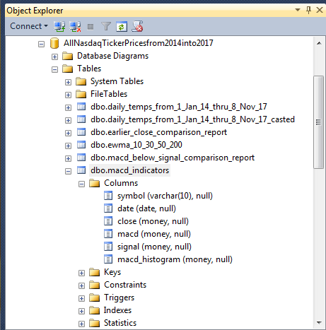
The following screen shot shows an Object Explorer view of the macd_indicators table in the AllNasdaqTickerPricesfrom2014into2017 database. As you can see, the table contains a column for each of the three MACD indicators (macd, signal, and macd_histogram). Additionally, there is a column of close values in the table as well. The values in each row are uniquely identified by their symbol and date column values.

There are 3266 distinct stock symbols in the database, but only a fraction of these symbols is well suited for use in this tip. The primary filtering objective is to find investment grade stocks with substantial amounts of historical data. The following four criteria discovers a total of 245 stocks that meet all primary filtering objective criteria from within the AllNasdaqTickerPricesfrom2014into2017 database. The result set is ordered by the difference between the maximum and minimum close prices for historical close prices within each symbol, and each symbol is assigned a row number. This facilitates the selection of two relatively matched sets of stock symbols based on odd or even row number values.

The criteria for investment grade securities that are also good for testing purposes are briefly described below.

• Each stock symbol must have a minimum number of daily traded shares of 100,000. This requirement is to ensure that selected stocks are easily traded.
• Each stock was required to have data for a minimum of 900 trading days. This ensures that each stock symbol has plenty of data for which to calculate MACD indicator values.
• All stock symbols must have their most recent trading day on either November 7 or 8, 2017. The data were collected from Yahoo Finance while updates for the current day of trading (November 8, 2017) were still in progress. So, the last trading day could be November 7 or 8, 2017. If a stock has historical data for neither of these two days, then it is not traded on a daily basis, and the stock is excluded from consideration for this tip.
• The minimum close price for a stock symbol must be at least $5. Institutional investors, which control the bulk of share transactions, tend to avoid stocks with a share price below $5.

The following script draws the sample of 245 investment grade stock symbols with substantial historical data in the AllNasdaqTickerPricesfrom2014into2017 database. Notice that each row is assigned a row_number value and that row_number values are based on the difference of the maximum close price less the minimum close price. The ordered stock symbols with associated filtering data are saved in the ##symbol global temporary table. Two queries at the end of the following script show how to specify a sample of the top ten symbols with either odd or even valued row numbers. These two sets of symbols are comparable in terms of the filtering criteria.

If you run the script, you will discover a symbol value of PCLN. This symbol is for a company named PriceLine.com at the time that the sample was drawn from the NASDAQ exchange website (nasdaq.com). Shortly after the sample was drawn, the company changed its name to Bookings Holding with a symbol value of BKNG. I have two reasons for pointing this out. First, the PCLN symbol is no longer listed on the NASDAQ stock exchange; the company is now represented by the BKNG symbol. Second, you should understand that historical stock data is constantly evolving as circumstances change. This real-world feature is one reason historical price and volume data represents such a good source for demonstrating database development techniques.

begin try
drop table ##symbol
end try
begin catch
print '##symbol not available to drop'
end catch

-- put symbol list into ##symbol
select 
* 
into ##symbol
from
(
-- returns 245 symbols matching criteria from inner query
select *
from
(
-- set of symbols with 
--		minimum volume > 100000
--		most recent date of '2017-11-07' or '2017-11-08'
--		at least 900 time series rows of data
--		minimum close price of $5
-- 245 symbols meet the criteria
-- row_number order is desc on max_close-min_close
select 
row_number() over (order by max_close-min_close desc) row_number, *
from
(
-- 3266
select
 symbol
,min([close]) min_close
,max([close])  max_close
,min(volume)  min_volume
,min(date)    min_date
,max(date)    max_date
,count(*)     number_recs
FROM [AllNasdaqTickerPricesfrom2014into2017].[dbo].Results_with_extracted_casted_values
group by symbol
) for_outer_query
where 
min_volume > 100000
and max_date >= '2017-11-07'
and number_recs > 900
and min_close > 5
) for_odd_even_row_number

) for_##symbol_global_temp_table

-- display top 10 odd sample symbols from those meeting criteria
-- ordered by difference between max_close and min_close
select top 10 * from ##symbol where (row_number % 2) = 1 order by row_number

-- display top 10 even sample symbols from those meeting criteria
-- ordered by difference between max_close and min_close
select top 10 * from ##symbol where (row_number % 2) = 0 order by row_number

Identifying start and end dates for MACD up cycles

This tip focuses on how the three MACD indicators can point to trading dates that are better on average than other trading dates for owning or not owning a stock. This tip designates the start date for an MACD up cycle as the first trading date where the MACD value moves from below zero to above zero. The hold duration for a stock is arbitrarily specified as twenty days from the buy date. This relatively short hold period is long enough to capture many close price changes for each stock over the four-year time span for which historical stock prices and MACD indicators are available in the AllNasdaqTickerPricesfrom2014into2017 database. In fact, this relatively short hold period probably understates the magnitude of the gain in MACD up cycles because larger price gains are associated with longer MACD up cycles. This understatement is not important because the goal of this tip is to highlight how each of the three MACD indicators impact stock price movement in the twenty days after the MACD crosses from below to above its centerline value.

The following script shows some T-SQL code for finding the start and end dates for holding stocks among those symbols with an odd row number value. The query populates a fresh copy of the ##macd_gt_0_cycles table with a row for each up cycle. The up cycles are for the ten stock symbols with odd row number values in the ##symbol table.

• The for_macd_lag_1 sub-query pulls start and end data for holding periods from the macd_indicators table.
  • A nested sub-query is, in turn, dependent on another query from the ##symbol table.
  • The sub-query in the from clause designates the top ten stock symbols with odd row numbers.
• The column values for each row in the for_macd_lag_1 sub-query result set designate start and end values for each up cycle.
  • For example, the date and close column values designate the start date and close price of each up cycle.
  • The date_lead_20 and close_lead_20 designate the end date and close price for each up cycle.
  • The symbol column value denotes the stock symbol for which start and end date and close price values apply.
  • The macd_gt_0_cycle# is a row_number value that uniquely identifies each up cycle.
• The select statement from the outermost query pumps the unique up cycle identifier values along with the column values from the for_macd_lag_1 sub-query result set into the ##macd_gt_0_cycles table.
• The where clause in the outermost query specifies the filter to extract the start of each up cycle.
• The final select statement displays the values in the ##macd_gt_0_cycles table.

use AllNasdaqTickerPricesfrom2014into2017
go

begin try
drop table ##macd_gt_0_cycles
end try
begin catch
print '##macd_gt_0_cycles not available to drop'
end catch


-- for macd > 0 crossover cycles
select row_number() over (order by symbol, date) macd_gt_0_cycle#, *
into ##macd_gt_0_cycles
from
(
select 
 symbol
,[date]
,lead([date],20) over (order by symbol, [date]) date_lead_20
,[close]
,lead([close],20) over (order by symbol, [date]) close_lead_20
,lag(macd,1) over (order by symbol, [date]) macd_lag_1
,macd
from macd_indicators
where 
symbol in 
(
-- top 10 odd sample symbols from those meeting criteria
-- ordered by difference between max_close and min_close
select top 10 symbol from ##symbol where (row_number % 2) = 1 order by row_number
)
and date != '2017-11-08'  -- cannot have a cycle that starts on the last date
) for_macd_lag_1
where macd_lag_1 < 0 and macd > 0

order by symbol, date

select * from ##macd_gt_0_cycles order by symbol, date

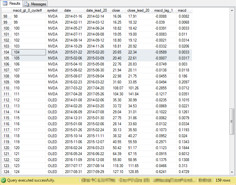
The following screen shot displays an excerpt from the output of the preceding select statement. There are two sets of rows in the output - one for the NVDA symbol and another for the OLED symbol; both symbols represent technology hardware manufacturing companies.

• The date column values denote the beginning of an up cycle for a symbol. On an up cycle date, the macd column value rises above zero from a preceding value (macd_lag_1) that is below zero.
• The date_lead_20 column values indicate the twentieth trading date after the up cycle begins. Trading does not occur on weekend days as well as during a select set of holidays.
• The close and close_lead_20 column values are, respectively, the close price for a symbol at the beginning and twentieth trading day after the beginning of an up cycle.
• Each symbol can have multiple up cycles. The up cycles are uniquely identified by the values in the macd_gt_0_cycle# column.
• Up cycles can occasionally overlap with one another. For example, the up cycle on row 104 ends on 2015-02-20 which is after the start of the up cycle on row 105 on 2015-02-06.
• The number in the lower right portion of the screen shot border reveals that there is a total of 159 up cycles for the ten symbols in the odd symbol set.

Joining the macd_indicators rows with the ##macd_gt_0_cycles rows

To perform an analysis on the path of close prices within up cycles and track the associated movements of MACD indicator values, we need a joined result set based on the macd_indicators table and the ##macd_gt_0_cycles table. The joined result set additionally needs other columns with values for correlating changes in MACD indicator values to close price changes.

The following script illustrates the basics for how to join macd_indicators table rows with ##macd_gt_0_cycles table rows. Notice that the inner join between the two tables matches rows on three criteria. This code sample is not actually used in the solution, but it is a basis for more complex code that is used in the solution to accomplish the join and perform other functions as well.

• The symbol column value must match between the two tables.
• The date column value from the macd_indicators table must be greater than or equal to the date column value from the ##macd_gt_0_cycles table.
• The date column value from the macd_indicators table must be less than or equal to the date_lead_20 column value from the ##macd_gt_0_cycles table.
• The final order by clause references symbol, macd_gt_0_cycle#, and date from the macd_indicators table; this sort order properly arranges the same data in multiple up cycles when the end of one up cycle overlaps with the start of another cycle.

-- join detailed macd_indicator rows with 
-- ##macd_gt_0_cycles rows
-- to show macd indicators and close prices 
-- for trading days within each cycle

select ##macd_gt_0_cycles.*, macd_indicators.*
from macd_indicators
inner join
##macd_gt_0_cycles
on 
macd_indicators.symbol = ##macd_gt_0_cycles.symbol
and macd_indicators.date >= ##macd_gt_0_cycles.[date]
and macd_indicators.date <= ##macd_gt_0_cycles.date_lead_20

order by ##macd_gt_0_cycles.symbol, macd_gt_0_cycle#, macd_indicators.date

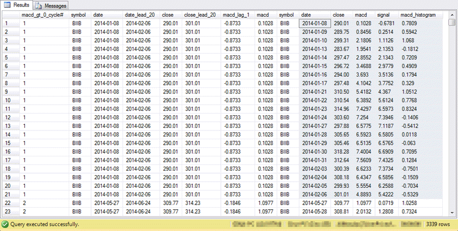
The following screen shot shows an excerpt from the preceding select statement.

• There are twenty-one rows for each up cycle; these rows start with a beginning row in which the MACD value crosses the centerline followed by data for the next twenty trading days.
• All twenty-one rows for the first up cycle show, and the first two rows for the second up cycle show.
• The data in the first seven columns are from the ##macd_gt_0_cycles table; the remaining columns are from the macd_indicators table.
• The rows from the macd_indicators table appear in date order within an up cycle from the ##macd_gt_0_cycles table.

The next script builds on the demonstration code in the preceding script.

• This code creates and populates a fresh copy of the ##macd_gt_0_accounting table with the joined data based on the design in the preceding script.
  • A try…catch block at the top of the script drops any prior version of the ##macd_gt_0_accounting table.
  • The into keyword just before the from clause inserts the result set from the select statement into the ##macd_gt_0_accounting table.
• Additionally, various accounting fields are added to facilitate an analysis of the joined data. The accounting fields are to facilitate tracking changes from the beginning trading date for an up cycle as well as from the preceding trading day in an up cycle. These changes are monitored for
  • Close price changes
  • Value changes for MACD indicators
• It is necessary or sometimes just helpful to re-name selected source data columns from the joining of the macd_indicators and ##macd_gt_0_cycles tables. This re-naming distinguishes similarly or identically named columns from the original data source in the two different tables.
  • For example, there are columns named date in both the macd_indicators and ##macd_gt_0_cycles tables.
  • However, the two columns serve different roles in each table.
  • Therefore, these identically named columns are assigned distinct aliases in the joined result set.
    • The date column from the macd_indicators table is re-named date_from_indicators.
    • The date column from the ##macd_gt_0_cycles table is re-named date_from_cycles.

There are two main types of accounting fields based on macd indicator values.

• Two accounting fields characterize the value of the MACD relative to one of two other values.
  • The macd_gt_0 accounting field can have one of three values.
    • It is assigned a null value when a trading day is the first day in an up cycle. This assignment is used as a marker for the beginning row in up cycles. As you'll see, this row serves as a reference point for certain percentage change metrics.
    • It is assigned a value of one for any symbol's trading date when the MACD for that date is greater than zero.
    • It is assigned a value of zero otherwise.
  • The macd_gt_signal accounting field is processed similarly.
    • If it is the beginning row in an up cycle, then it is assigned a null value.
    • If the macd value exceeds the signal value, then it is assigned a value of one.
    • Else, it is assigned a value of zero.
• Three accounting fields assess the percentage change from the preceding day in an up cycle.
  • The close_change_from_yesterday field is calculated as the change in close price from the preceding trading day in an up cycle for a symbol except for the beginning date in an up cycle; this field is null for the beginning date in an up cycle for a symbol.
  • The macd_change_from_yesterday field is calculated as the change in MACD value from the preceding trading day in an up cycle for a symbol for all days except the beginning date in an up cycle; this field is null for the beginning date in an up cycle for a symbol.
  • The histo_change_from_yesterday field is calculated as the change in the MACD histogram value from the preceding trading day in an up cycle for a symbol for all days except the beginning date in an up cycle; this field is null for the beginning date in an up cycle.

begin try
drop table ##macd_gt_0_for_accounting
end try
begin catch
print '##macd_gt_0_for_accounting is not available to drop'
end catch

-- joined #macd_gt_0_cycles rows with macd_indicators rows
-- with accounting metrics added
select 

-- start of accounting metrics fields

 ##macd_gt_0_cycles.[date] first_date
,first_value(macd_indicators.[close]) over (partition by macd_gt_0_cycle# order by macd_gt_0_cycle#) first_close
,macd_indicators.[close] close_today
,##macd_gt_0_cycles.close_lead_20 close_last
,macd_indicators.[close] - first_value(macd_indicators.[close]) over (partition by macd_gt_0_cycle# order by macd_gt_0_cycle#) close_change_from_first
,
round(
(macd_indicators.[close] - first_value(macd_indicators.[close]) over (partition by macd_gt_0_cycle# order by macd_gt_0_cycle#))
/
first_value(macd_indicators.[close]) over (partition by macd_gt_0_cycle# order by macd_gt_0_cycle#) *100
,2) percent_close_change_from_first
,
case
	when macd_indicators.date = ##macd_gt_0_cycles.[date] then NULL
	when macd_indicators.macd > 0 then 1
	else 0
end macd_gt_0
,case
	when macd_indicators.date = ##macd_gt_0_cycles.[date] then NULL
	when macd_indicators.macd > macd_indicators.signal then 1
	else 0
end macd_gt_signal
,
case
	when macd_indicators.date = ##macd_gt_0_cycles.[date] then NULL
	else 
	macd_indicators.[close] - lag(macd_indicators.[close],1) over (partition by macd_indicators.symbol order by macd_indicators.date)
end close_change_from_yesterday
,
case
	when macd_indicators.date = ##macd_gt_0_cycles.[date] then NULL
	else 
	macd_indicators.macd - lag(macd_indicators.macd,1) over (partition by macd_indicators.symbol order by macd_indicators.date)
end macd_change_from_yesterday
,
case
	when macd_indicators.date = min(macd_indicators.date) over (partition by macd_gt_0_cycle# order by macd_gt_0_cycle#) then NULL
	else 
	macd_indicators.macd_histogram - lag(macd_indicators.macd_histogram,1) over (partition by macd_indicators.symbol order by macd_indicators.date)
end histo_change_from_yesterday

-- end of accounting metrics fields


-- start of re-named source data fields

,macd_indicators.symbol symbol_from_indicators
,macd_indicators.[date] date_from_indicators
,macd_indicators.[close] close_from_indicators
,macd_indicators.macd macd_from_indicators
,macd_indicators.signal signal_from_indicators
,macd_indicators.macd_histogram histogram_from_indicators
,##macd_gt_0_cycles.macd_gt_0_cycle#
,##macd_gt_0_cycles.symbol symbol_from_cycles
,##macd_gt_0_cycles.[date] date_from_cycles
,##macd_gt_0_cycles.date_lead_20 last_date
,##macd_gt_0_cycles.[close] close_from_cycles
,##macd_gt_0_cycles.macd_lag_1
,##macd_gt_0_cycles.macd macd_from_cycles

-- end of re-named source data fields

into ##macd_gt_0_for_accounting

from macd_indicators
inner join
##macd_gt_0_cycles
on 
macd_indicators.symbol = ##macd_gt_0_cycles.symbol
and macd_indicators.date >= ##macd_gt_0_cycles.[date]
and macd_indicators.date <= ##macd_gt_0_cycles.date_lead_20

order by ##macd_gt_0_cycles.symbol, macd_gt_0_cycle#, macd_indicators.date

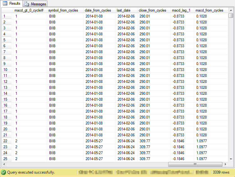
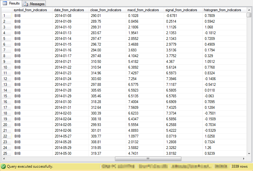
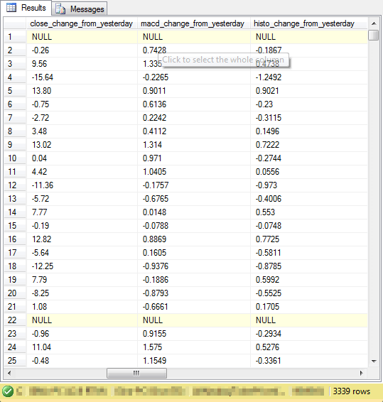
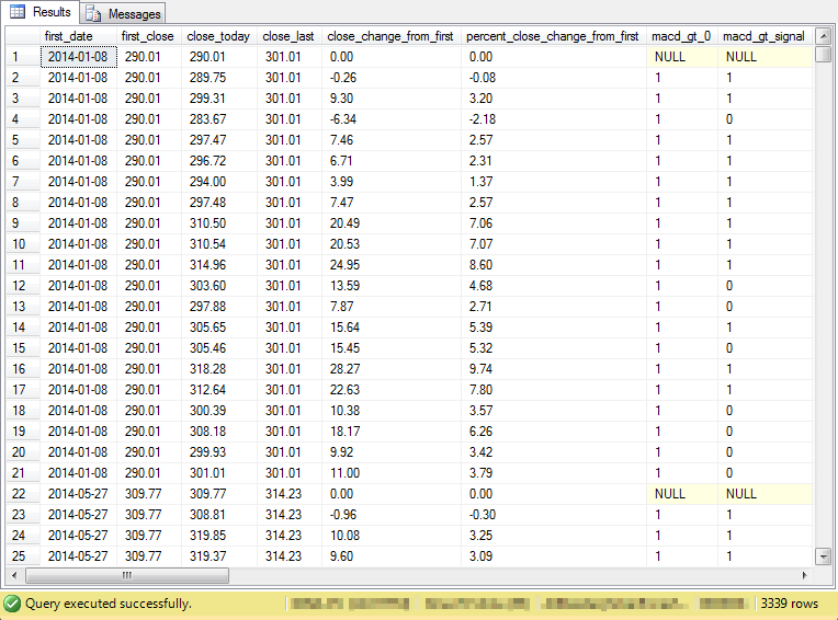
The preceding script to populate the ##macd_gt_0_for_accounting table has so many columns that they are not easily viewed in a single screen shot. Furthermore, there are natural groupings to the columns in the table. Therefore, the following four screen shots each display a subset of the columns for the first twenty-five rows in the table. As you can see from the border in each of the screen shots, there are total of 3,339 rows in the overall table. I often use a quantity such as this for unit testing my code.

• The first screen shot displays the columns from the ##macd_gt_0_cycles table. These columns are sometimes re-named, but they appear in the same order as the original ##macd_gt_0_cycles table.
• The second screen shot shows the columns from the macd_indicators table. These columns are again re-named, but they are otherwise the same as in the original macd_indicators table.
• The third screen shot shows a set of three accounting fields named: close_change_from_yesterday, macd_change_from_yesterday, and histo_change_from_yesterday. Each of these fields are defined in the description of the preceding script.
• The fourth screen shot presents data for summarizing the percent change in close price from the beginning of an up cycle through each of the remaining twenty trading days in an up cycle. This column is named percent_close_change_from_first. In a subsequent analysis, you'll see how to summarize the average percent_close_change_from_first for the combination of the macd_gt_0 and macd_gt_signal fields.

Category Analysis for macd_gt_0 and macd_gt_signal

If MACD reflects upward close price changes, then knowing a timeline for the relationship of close prices and macd_gt_0 and macd_gt_signal field values should help identify good dates for owning or not owning a stock. In general, you should own a stock when its close price is rising, and you should not own a stock when its close price is declining.

The combination of macd_gt_0 and macd_gt_signal field values can identify four times during which it may be beneficial to own or not own a stock. See below category names for four times based on these field values.

• Don't own a stock -- it's MACD is not greater than its Signal value (macd_gt_signal = 0) and its MACD is not above its centerline value (macd_gt_0 = 0)
• Consider owning a stock - its MACD value is above its Signal value (macd_gt_signal = 1) and its MACD is below its centerline value (macd_gt_0 = 0)
• Own a stock - its MACD is above its Signal value (macd_gt_signal = 1) and its MACD is above its centerline value (macd_gt_0 = 1)
• Consider not owning a stock - its MACD is below its Signal value (macd_gt_signal = 0) and its MACD is above its centerline value (macd_gt_0 = 1)

In the twenty-trading trading days after the beginning of potential up cycles based on the MACD switching from below its centerline to above its centerline, the MACD can

• Stay above the centerline for all twenty-trading days
• Fall immediately after the beginning to below the centerline and never rise above it
• Stay above the centerline value for a fraction of the twenty trading days

In each of these twenty trading days, the MACD value can be above or below the Signal value. Recall also that some twenty-day cycles end after the next twenty-day cycle starts. Therefore, it is possible for some days to belong to more than one up cycle.

The following script computes the average percent change in close price from the beginning of a cycle and the frequency of trading days by macd_gt_0 and macd_gt_signal values.

• The select list returns four values: macd_gt_0, macd_gt_signal, avg for average percent change from the beginning close price for a cycle, and obs for the count of the number of days in a category.
• The from clause designates the ##macd_gt_0_for_accounting table as the data source for the query; this global temporary table is computed by the preceding script.
• The group by clause aggregates source data based on the values of the macd_gt_0 field and the macd_gt_signal field.
• The having clause excludes any source data row with a macd_gt_0 value of null. This eliminates rows for the beginning row in up cycles from aggregated results.

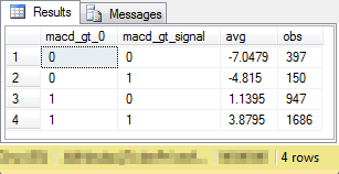
-- calculate the frequency of observations and average 
-- percent change in close price from the beginning 
-- of a cycle by macd_gt_0 and macd_gt_signal
-- category values
select 
 macd_gt_0
,macd_gt_signal
,avg(percent_close_change_from_first)  [avg]
,count(*) [obs]
from ##macd_gt_0_for_accounting
group by macd_gt_0, macd_gt_signal
having macd_gt_0 is not null

See below a screen shot of the query's result set in the Results tab. Notice the results are implicitly ordered by their macd_gt_0 and macd_gt_signal values because of the group by clause and actual values of the two category fields. The order of rows in the result does not match the ownership timeline, but each timeline point links to one pair of macd_gt_0 and macd_gt_signal values.

• The 0,0 field values denote the "Don't own" category.
• The 0,1 field values denote the "Consider owning" category.
• The 1,1 field values denote the "Own" category.
• The 1,0 field values denote the "Consider not owning" category.

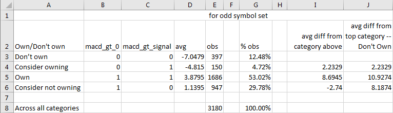
The next screen shot shows the results after copying raw output to Excel. Additionally, there is some minor processing of the copied results. These results are based on trading days for symbols with odd row numbers.

• Column A displays category names. Matching macd_gt_0 and macd_gt_signal field values appear in columns B and C, respectively.
• The average close percent relative to the beginning close (avg) for each category appears in column D.
• The number (obs) and percent of observations (% obs) for each category appear in columns E and G.
• The avg difference from the category above for MACD up cycles (avg diff from category above) appears in column I.
• The difference from the top category ("Don't own") in avg appears in column J (avg diff from top category - Don't Own).

Note that the greatest difference from the top category ("Don't own") is for the "Own" category. This difference is nearly eleven percentage points (10.9274). Also, the difference is positive indicating the percentage gain is nearly eleven percentage points higher on "own" category trading days than on "don't own" trading days. Furthermore, there is a rounded three percentage point drop (-2.74) on "consider not owning" trading days relative to "own" trading days.

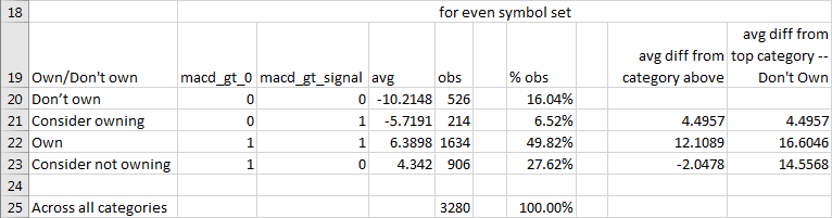
The next screen shot shows the same kind of results tabulated for symbols with an even row number. Although the tabulated outcomes are not identical for those based on trading days from the odd symbol set, the general pattern of key relationships is the same.

• The greatest difference in column J (avg diff from top category - Don't Own) is for the "Own" category relative to the "Don't own" category. The percentage point gain is over sixteen points for the "Own" category relative to the "Don't own" category.
• Also, column I (avg diff from category above) reports a modest drop of about two percentage points for the "consider not owning" category relative to the "own" category.

Linear regression analysis for estimating change in close from yesterday

The previous section confirmed the impact of the MACD and Signal values on stock close prices. The impact in the previous section was measured by the average percentage change in close price from a beginning close price for a stock in an MACD up cycle. This section switches the focus to the impact of MACD histogram values on stock close prices. The goal of this section is to evaluate how well changes in MACD histogram values from yesterday predict changes in close prices from yesterday. As a point of reference, the section also evaluates how well changes in MACD values from yesterday predict changes in close prices from yesterday.

This section draws from T-SQL code for a prior tip on how to compute coefficients of determination as well as regression slope and intercept estimates for a fitted line. The prior tip presented two stored procedures - one for calculating a coefficient of determination and another for calculating the slope and intercept of a fitted line. It is convenient to have these two stored procedures because it eliminates the need to copy values out of SQL Server to another application, such as Excel, for calculating the line of best fit and its goodness of fit. This convenience is especially valuable for this tip because we will use the slope and intercept values in other calculations from within SQL Server.

• The coefficient of determination is a goodness of fit measure for the relation of a set of x values to a set of y values.
• The slope for a fitted line defines how changes in the x variable value impact changes in the y variable value.
• The intercept represents an offset value for aligning computed y values based on slope times x values to observed y values.

This section demonstrates how to reference the two stored procedures from the prior tip with three columns of data from the ##macd_gt_0_for_accounting table.

• In the first regression line fit, close_change_from_yesterday field values are predicted based on histo_change_from_yesterday field values.
• In the second regression line fit, close_change_from_yesterday field values are predicted based on macd_change_from_yesterday field values.

Here's the script for implementing the first regression line fit.

• The script starts by creating a fresh copy of the ##temp_xy table. This table holds the x and y values for two stored procedures that compute the coefficient of determination as well as slope and intercept values.
• An insert…select statement pumps the histo_change_from_yesterday field values as x values and the close_change_from_yesterday field values as y values into the ##temp_xy table.
• Next, the ##r_squared_outputs table is created and populated with the output from the compute_coefficient_of_determination stored procedure. This stored procedure outputs the coefficient of determination based on the data in the ##temp_xy table.
• Finally, the compute_slope_intercept_correlation_coefficient stored procedure is invoked. The stored procedure estimates the slope and intercept for the fitted line. The sources for the stored procedure are the ##temp_xy and ##r_squared_outputs tables.

-- compute slope and intercept as well as goodness of fit
-- for regression of close_change_from_yesterday on 
-- histo_change_from_yesterday

-- create and populate ##temp_xy
begin try
drop table ##temp_xy
end try
begin catch
print '##temp_xy not available to drop'
end catch

create table ##temp_xy 
(
 --pkID integer identity(1,1) primary key,
 x float,
 y float
)
go

insert into ##temp_xy
select 

 histo_change_from_yesterday  -- this is for x
,close_change_from_yesterday  -- this is for y
from ##macd_gt_0_for_accounting
where macd_gt_0 is not null


-- select top 1000 * from ##macd_gt_0_for_accounting
-- select * from ##temp_xy

-- create a fresh copy of the ##r_squared_outputs
-- to store outputs from the stored procedure to
-- compute the coefficient of determinaton and 
-- correlation coefficient

begin try
drop table ##r_squared_outputs
end try
begin catch
print '##r_squared_outputs not available to drop'
end catch


create table ##r_squared_outputs 
(
 sum_of_y_sq_devs float
,sum_of_x_sq_devs float
,sum_of_xy_product_devs float
,correlation_coefficient float
,coefficient_of_determination float
)
go

-- Finally, invoke the compute_coefficient_of_determination
-- stored procedure followed by the compute_slope_intercept_correlation_coefficient
-- stored procedure
insert ##r_squared_outputs 
exec dbo.compute_coefficient_of_determination

exec dbo.compute_slope_intercept_correlation_coefficient

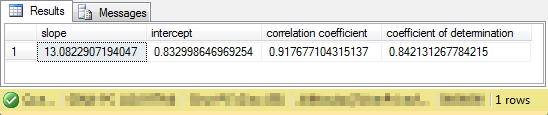
Here's the output from the preceding script. As you can see, the compute_slope_intercept_correlation_coefficient stored procedure returns a result set with a single row of values.

• The coefficient of determination value indicates that slightly in excess of eighty-four percent of the variance in close price changes from yesterday is explained by changes in MACD histogram values from yesterday.
• Furthermore, the line of best fit is defined by the values of slope * histo_change_from_yesterday + intercept.
• It is the computed y values that have .84 coefficient of determination with the observed y values where y values are close_change_from_yesterday field values.

To compute the line of best fit and coefficient of determination for close_change_from_yesterday field values versus macd_change_from_yesterday field values all you need to do is modify the line for specifying x values in the preceding script. For example, make the following swap. The macd_accounting_for_odd_symbols.sql script file that is available for download with this tip has the complete version for both pairs of x and y values so that you can verify the outcomes without any swapping of lines.

• Replace: histo_change_from_yesterday -- this is for x
• With: macd_change_from_yesterday -- this is for x

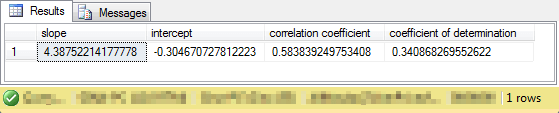
Here's the slope, intercept, and coefficient of determination (along with the correlation coefficient) for close_change_from_yesterday field values estimated by macd_change_from_yesterday. As you can see, the percentage of explained close_change_from_yesterday field value variance is around thirty-four percent. This is a substantial decline (around fifty percentage points of explained variance) from the prediction of close_change_from_yesterday field values based on histo_change_from_yesterday field values.

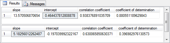
The preceding two screen shots show the slope, intercept, and coefficient of determination (along with the correlation coefficient) for the regression of close_change_from_yesterday separately on histo_change_from_yesterday and macd_change_from_yesterday. The results set in each screen shot is for the trading days associated with symbols having an odd row number in the ##symbol table. The next screen shot shows a Results tab with analogous results sets for symbols having an even row number in the ##symbol table.

• The top pane shows the result set for the regression among symbols with even row numbers for close_change_from_yesterday values on histo_change_from_yesterday values.
  • The coefficient of determination is slightly greater than .88. This value is highly similar to the one calculated for the trading days for odd symbols (.84).
  • Even more importantly, the slope for the trading days for even symbols closely matches the values calculated for odd symbols.
  • The match for the intercept values is not as close, but the size of this term plays a smaller role in determining predicted values so the difference is correspondingly less important.
• The bottom pane shows the result set for the regression among symbols with even row numbers for close_change_from_yesterday values on macd_change_from_yesterday values.
  • Again, the coefficient of determination for the even symbols (.40) generally matches the coefficient of determination for odd symbols (.34).
  • While the slope and intercept values for the data for even symbols generally match those for odd symbols, the correspondence is relatively less tight for the regression on macd_change_from_yesterday values versus histo_change_from_yesterday values.

Cross validation of linear regressions for odd versus even symbols

Up to this point, the regression analysis has created two slightly different models for estimating close_change_from_yesterday values versus histo_change_from_yesterday values. The regression model based on the data for odd symbols has a coefficient of determination of about .84 while the coefficient of determination is about .88 for the model based on the even symbols. However, is the slight difference between these two outcomes a result of the fitted line models or the data? Additionally, can you use one model to predict close_change_from_yesterday values based on histo_change_from_yesterday from both samples of symbols?

One way to answer these questions is to use the model based on odd symbols to predict y values for the data with even symbols. In like manner, you can use the model based on even symbols to predict y values for data with odd symbols. This is an example of cross validation in that each model is tested with the data for the other sample of symbols. You are validating the models across different data sets. This is why we call it cross validation.

The following script demonstrates cross validation of the model developed based on the data for even symbols with the data for odd symbols.

• The slope and intercept from the model based on data for even symbols are, respectively, 13.570506870654 and 0.464437812808878.
• The first select statement returns three columns of data for unit testing purposes.
  • The first column contains histo_change_from_yesterday values for the odd sample.
  • The second column contains close_change_from_yesterday values for the odd sample.
  • The third column contains predicted close_change_from_yesterday values for the odd sample based on the slope and intercept values from the model developed for data from symbols with even row numbers.
• The insert…select statement compiles a result set for insertion into the ##temp_xy table.
  • The x variable is populated with predicted close_change_from_yesterday values based on slope and intercept values calculated from the even symbol data. The predicted values are computed as the slope times the histo_change_from_yesterday values for the odd sample plus the intercept.
  • The y variable is populated with close_change_from_yesterday values for the odd symbols.
  • This formulation regresses the observed close_change_from_yesterday values for the odd symbol data on the predicted close_change_from_yesterday values.
• The next major steps are to successively invoke the compute_coefficient_of_determination and compute_slope_intercept_correlation_coefficient stored procedures.

-- do cross validation with model for even symbols
-- slope from even sample: 13.570506870654
-- intercept from even sample: 0.464437812808878

-- The predicted values with odd sample parameters 
-- have a coefficient of determination of .88 with 
-- close_change_from_yesterday values from the even sample
-- The predicted values from the even sample also
-- has a coefficient of determination of .88

select 
 histo_change_from_yesterday  -- this is for x
,close_change_from_yesterday  -- this is for y
,13.570506870654*histo_change_from_yesterday + 0.464437812808878 predicted_y

from ##macd_gt_0_for_accounting
where macd_gt_0 is not null


-- now use predicted_y values for estimating the observed y values

delete ##temp_xy 

insert into ##temp_xy
select 
 13.570506870654*histo_change_from_yesterday 
 + 0.464437812808878 -- predicted_y serves as x value
,close_change_from_yesterday  -- this is for y

from ##macd_gt_0_for_accounting
where macd_gt_0 is not null


delete ##r_squared_outputs

-- Finally, invoke the compute_coefficient_of_determination
-- stored procedure followed by the compute_slope_intercept_correlation_coefficient
-- stored procedure
insert ##r_squared_outputs 
exec dbo.compute_coefficient_of_determination

exec dbo.compute_slope_intercept_correlation_coefficient

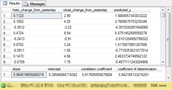
The next screen shot displays selected output from the preceding script.

• In the top pane, there is an excerpt of the three columns for unit testing.
  • The first column shows the observed histo_change_from_yesterday values for the odd sample of symbols.
  • The second column presents the close_change_from_yesterday values for the odd sample of symbols.
  • The third column presents the calculated results for the predicted close_change_from_yesterday values based on the slope and intercept for the model based on even symbols.
• The bottom pane displays the output from the compute_slope_intercept_correlation_coefficient stored procedures. This model output is for the prediction of the observed close_change_from_yesterday values for the odd sample of symbols based on the predicted values.
  • The slope is for multiplication times the predicted_y value.
  • The intercept value is a constant for addition to the product of the slope times the predicted_y value.
  • The coefficient of determination is the percent of explained variance for observed close_change_from_yesterday values versus the model outcomes based on the slope and intercept.
  • Notice that the percent of explained variance is eighty-four percent, which matches the original coefficient of determination for predicting close_change_from_yesterday values from histo_change_from_yesterday values for the odd sample of symbols.

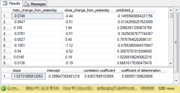
The next screen shot shows the output for estimating predicted close_change_from_yesterday values for the even symbol sample based on a prediction model using slope and intercept derived from using data for the odd symbol sample. For your easy reference, the macd_accounting_for_even_symbols.sql file, which is available as one of the files with this tip, has the full script for generating the results shown below.

From a prediction perspective, the most important value may be the one for the coefficient of determination. Notice that the value is slightly more than .88. Recall that a coefficient of determination of .88 was also calculated for the model of close_change_from_yesterday values versus histo_change_from_yesterday for the even symbol sample. Therefore, whether we use the model from the odd sample or the model from the even sample, we get the same eighty-eight percent of the variance explained in the even sample.

Based on these results, two conclusions are supported.

• You can use either model to predict close_change_from_yesterday values in both samples. Each model has the same coefficient of determination of .84 for the odd sample data and .88 for the even sample data.
• Given that you use least squares to estimate a best fit model for each sample, the sample, and not the calculated slope and intercept estimates, determines the coefficient of determination for the fit of either model.

Next Steps

There are four steps necessary for trying out the scripts from this tip.

• First, you need to download the backup file for the AllNasdaqTickerPricesfrom2014into2017 database from this tip. The database includes NASDAQ historical price and volume data.
• Second, you need to download a script file from this other prior tip on how to create and populate the macd_indicators table for all stocks in the database.
• Third, you need to download the script file from this tip on a T-SQL starter statistics package for the AllNasdaqTickerPricesfrom2014into2017 database. The code to create stored procedures are essential for the steps calculating fitted lines and goodness of fit measures.
• Fourth, download the files for this tip from this link. The link will enable you to duplicate all the metrics and statistics reported in this tip. Even if you do not care about stock prices relative to macd indicators, these scripts provide valuable code demonstrating the cross validation technique for verifying linear regression models. If you care about growing your data science skills, it would be beneficial to gain proficiency on topics such as this.

About the author

Rick Dobson is an author and an individual trader. He is also a SQL Server professional with decades of T-SQL experience that includes authoring books, running a national seminar practice, working for businesses on finance and healthcare development projects, and serving as a regular contributor to MSSQLTips.com. He has been growing his Python skills for more than the past half decade -- especially for data visualization and ETL tasks with JSON and CSV files. His most recent professional passions include financial time series data and analyses, AI models, and statistics. He believes the proper application of these skills can help traders and investors to make more profitable decisions.

This author pledges the content of this article is based on professional experience and not AI generated.

View all my tips