T-Test Add-on for the SQL Statistics Package

By: Rick Dobson   |   Comments   |   Related: > TSQL

Problem

MSSQLTips.com previously published a helpful introduction for doing statistics with SQL Server T-SQL code. Please update the SQL statistics package to allow more and different kinds of t tests. Also, enable the package to lookup automatically the statistical significance of computed t values. Finally, demonstrate how to compute an F test to assess if the variance in one group is different than another.

Solution

An important element of many data science projects is the capability to perform statistics. As the popularity of data science projects within organizations continues to grow, it becomes increasingly beneficial for SQL Server professionals to have an integrated set of stored procedures for implementing analyses of data in SQL Server instances. These stored procedures should be easy to use, add on to, and expand as data science requirements evolve. This tip builds on several prior tips in moving towards the fulfillment of these goals.

Here's some history on the topic.

• The T-SQL Starter Statistics Package for SQL Server tip initially presented a SQL starter statistics package available from MSSQLTips.com.
• This general topic was revisited in a follow-up overview tip on the role of statistics in data science projects and how to implement statistics in SQL Server.
• This tip extends the starter statistics package by adding new functionality relating primarily to t tests. A t test is very commonly used to assess whether the average of one group of values is statistically different from another group of values or a standard value.

This tip extends the SQL starter statistics package with new stored procedures, tables, and additional capabilities that remove the need to reference external resources for looking up the statistical significance of computed t values.

• Some new SQL Server tables based on Excel built-in statistics functions remove the need for manually looking up the statistical significance of computed t values. Understanding the derivation of these tables can grow your knowledge of Excel functions used to populate critical values in the lookup tables and generally enhance your understanding of how to perform statistics with SQL.
• You will discover within this tip, SQL code for implementing five different variations of a t test. Each section for a t test begins with a short statement explaining when to use it. Each t test presentation includes a stored procedure for implementing the t test, sample data for demonstrating the t test, and some SQL code illustrating the running of the stored procedure with the sample data.
  • The sections for two previously presented stored procedures highlight how to add on the capability for automatically looking up whether computed t values are statistically different.
  • This tip also describes three additional types of t tests not included in the SQL starter statistics package.
  • The stored procedures for the freshly demonstrated t tests along with the original two t tests equip you with a wide range of statistical tools for evaluating the differences of means with the SQL statistics package.
• Finally, this tip introduces the package's first F test. In the context of this tip, the F test allows you to statistically verify if the variances for two sample groups of scores are from populations with the same or different variances. This capability is important because it can help you decide which of two different t tests to use for evaluating the differences between two means from distinct groups.

A framework for the statistics package

The initial release of the SQL statistics package featured two SQL Server objects.

• A temporary table for holding the input data for which the package generates a statistical value, such as a computed t value or the median for a group of scores. The layout of the temporary table can vary from one statistical analysis technique to the next.
• A stored procedure for performing the computations for a statistic. The stored procedure performs one or more computations to calculate a computed value based on the data in a temporary table.

With these two objects, any SQL professional should be easily able to use the SQL statistics package to perform statistics. Just follow these steps.

• Discover the stored procedure for the statistical technique that needs to be implemented.
• Populate the temporary table for the stored procedure that implements the desired statistical method.
• Run the stored procedure and use or examine the output.

Here's some pseudo code for the stored procedures used to compute statistics in this tip. The original statistics package did not have any input parameters, but all the stored procedures in this add-on to the original package require one or more input parameters. This add-on to the original SQL statistics package performs some of its calculations by

• embedding a stored procedure from the original package into a new stored procedure or
• creating a new stored procedure from scratch that enables additional features not available with the SQL starter statistics package

create procedure stored_procedure_name input parameter(s)
as
begin
	set nocount on;

------------------------------------------------------------------------------------
Place your debugged code here for a statistic and whatever associated values you want to 
output from your stored procedure.
------------------------------------------------------------------------------------

	return

end

The package relies on the population of global temporary tables with sample values for demonstrating how to run a t test by invoking a stored procedure. A global temporary table facilitates development and testing because it permits debugging a script in one SSMS tab and then copying the finished code into another tab with a collection of stored procedures for performing different kinds of statistical tests. A professional and/or enterprise SQL statistics package may benefit from using another SQL Server object for storing the data for a stored procedure. For example, you can consider local temporary tables, table variables, common table expressions, or permanent SQL Server tables.

The original SQL statistics package tip and this add-on tip were tested and developed inside the AllNasdaqTickerPricesfrom2014into2017 database; see here and here for more about this database. At present, you will need to manually copy stored procedures and some lookup tables to another database if you want to run the code from within another database. As the scope of the SQL statistics package grows, future tips may address using the package with any database without the need for copying stored procedures and tables between databases.

Computing and saving lookup tables containing critical values

The degrees of freedom for a computed t value or a computed F value can be looked up in a table of critical t or F values to assess if the computed t or F value is statistically significant in a one-tailed test or a two-tailed test. The type of test you use (two-tailed or one-tailed) depends on your null and alternative hypotheses.

• You should use a two-tailed test if it just matters that the two means are different, but it does not matter that one mean is either greater or less than the other mean. In this kind of test:
  • The null hypothesis is that the means are the same.
  • The alternative hypothesis is that the means are not the same, and it does not matter which mean is greater than the other.
  • This type of test is common when doing exploratory data analysis, and you have no a priori reason for believing that one group's mean is greater than another.
• You should use a one-tailed test if it does matter that one mean is greater than the other mean.
  • For example, if you are testing two different web page designs (a new one versus an old one), you may care which one generates the largest dollar amount of orders. In this case, it matters critically for whether to switch to the new page design if the dollar volume for the new page is greater than the dollar volume for the original page.
  • The null hypothesis is that the new page does not generate a larger dollar volume gain.
  • The alternative hypothesis is the new pages does generate a larger dollar volume.
• In addition to one-tailed and two-tailed t tests, this tip also demonstrates two-tailed F tests for assessing if the variance for one group is different than the variance for another group.
  • The null hypothesis is usually that the variances are the same in both groups.
  • The alternative hypothesis is that the variances are different, but it does not matter which variance is greater than the other.
  • This test for the equality of variances between two samples can indicate which t test to use for assessing if sample means are the same or different.

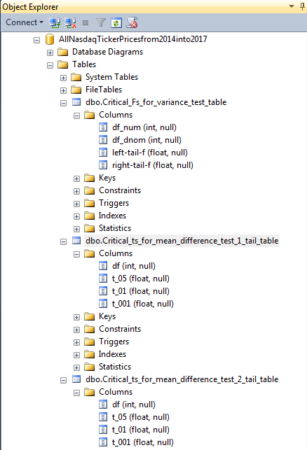
The following screen shot shows three tables of critical test values in the AllNasdaqTickerPricesfrom2014into2017 database. By comparing a computed t or F value to a critical t or F value based on the degrees of freedom of the computed test value, you can confirm if a computed t or F is statistically significant at some probability level. The first table is for critical F values. The second and third tables are for critical t values for one-tailed and two-tailed tests, respectively.

The design of the tables of critical values may differ depending on the type of test and how you want to assert the probability of a result being statistically significant.

• The two tables of critical values for evaluating computed t values have four columns each.
  • The first column is for degrees of freedom (df) values, which is typically based on the sample size for one or two groups of data values.
  • The three remaining columns are for different probability levels of assessing the difference between one sample mean and another or between a sample mean and a standard value.
    • A common minimum probability level is .05, which means that there are 5 chances in one hundred that a difference of this size could occur without there being a difference between a sample mean and a comparison value.
    • If a difference is significant at .01 or .001 probability levels, then the likelihood of obtaining that computed t value by chance is correspondingly rarer.
• The table of critical F test values is designed specifically for testing if there is a difference in the variances between two groups.
  • The computed F value for this kind of test is based on the ratio of the variance within one group to the variance within another group. Each sample or group can have the same or different sample sizes.
    • The degrees of freedom for the numerator in a ratio is denoted by df_num, and the degrees of freedom for the denominator in a ratio is denoted by df_dnom.
    • In either degrees of freedom, the sample size less one designates the degrees of freedom for a sample.
  • The F probability distribution, unlike the t probability distribution, is asymmetrical.
    • The absolute value of a computed t value can be compared to the same critical t value no matter which group has the larger mean.
    • In contrast, the computed F values need to be compared to different critical F values for each side of a two-tailed test. This is why the Critical_Fs_for_variance_test_table object has two separate columns of critical values.
      • If the computed F value is either less than or equal to the critical left-tail-f value or greater than or equal to the critical right-tail-f value, then the variances are different at the .05 probability level.
      • The critical F values table does not offer different probability value levels because if the variances are different at the .05 probability level, then that is sufficient to use one t test versus the other for comparing the difference between the means.

The next screen shot shows a pair of excerpts from the one-tailed and two-tailed critical t value tables. There are two hundred fifty rows in each of the tables, but just the first twenty-two rows are excerpted for the screen shots.

• The critical t values decline as the degrees of freedom (df) increase. It is easier to detect differences as the sample sizes for compared groups grow.
• The critical t values increase as the probability level rises from .05 through .001. It takes bigger differences to confirm a statistically difference at the .001 probability level than at the .05 probability level.
• For the same degrees of freedom (df) and probability level, the two-tailed critical t values are larger than the critical t values for a one-tailed test. In this sense, it is easier to confirm that group means are different for a one-tailed test than for a two-tailed test.

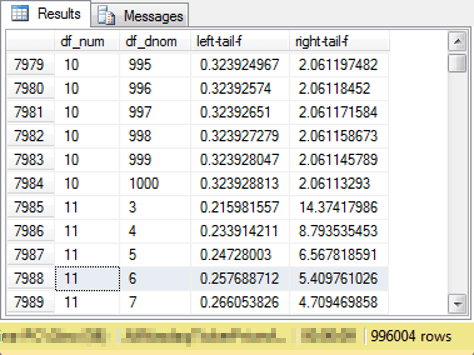
The next screen shot shows an excerpt from the F critical values lookup table in the database named AllNasdaqTickerPricesfrom2014into2017. Computed F values based on sample data are compared to critical F values to assess if an outcome is statistically significant. For this tip, the computed F value derives from the ratio of two sample variances.

• Recall that the df_num column value and df_dnom column value represent, respectively, the degrees of freedom for a F computed value.
• The left-tail-f column value represents a critical F value. Computed F values less than or equal to the left-tail-f column value qualify as statistically significant at the .05 level. In other words, the null hypothesis is rejected.
• The right-tail-f value represents another critical F value. Computed F values greater than or equal to the right-tail-f column value qualify as statistically significant at the .05 level. In other words, the null hypothesis is rejected.
• Computed F values that are greater than the left-tail-f column value and less than the right-tail-f value result in the acceptance of the null hypothesis, which for this tip corresponds to there being no significant difference in the variances between the two samples.

The expressions for computing critical t and F values can be complex. Beyond that, fully understanding the expressions for computing critical t and F values involves developing an appreciation of the distinction between probability density functions and cumulative probability density functions (for example, see here, here, here, and here).

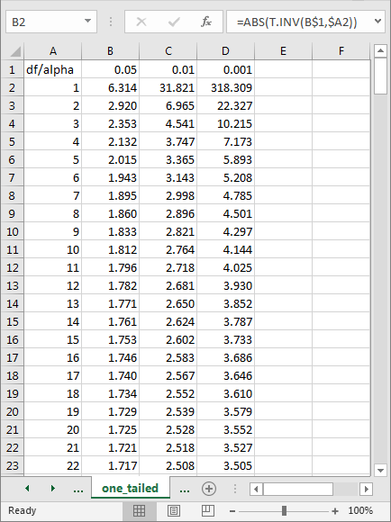
Happily, there is an easier way for users of Microsoft software to derive critical t and F values; this tip relies on the T.INV.2T Excel function for calculating critical t values. Microsoft Excel includes multiple built-in functions for computing critical values for multiple kinds of statistical functions. For example, the following spreadsheet shows an excerpt with critical t values from a worksheet tab named one-tailed.

• Start your review by confirming that the values in this table correspond to those for the one-tailed critical t values shown above.
• Therefore, the column A values represent df values and column B, C, and D values represent critical t values for .05, .01, and .001 probability levels.
• The cursor rests in cell B2, which denotes a critical t value for a computed t value with a df value of one and a probability level of .05.
• The expression in cell B2 is =ABS(T.INV(B$1,$A2)). This expression links the cell to a df value from cell A2 and the probability level in cell B1.
• The full worksheet tab has critical t values based on the formula for df values from one through two hundred fifty at probability levels of .05, .01, and .001.
• By switching the expression in cell B2 to =T.INV.2T(B$1,$A2), you can compute the comparable critical t values for a two-tailed t test. The two-tailed critical t values for df values one through two hundred fifty at .05, .01, and .001 probability levels are in another worksheet tab named two-tailed.
• Both the one-tailed and two-tailed tabs reside in an Excel worksheet file named "critical t values from excel functions". This file is available for download with this tip.
• After computing critical t values in Excel, you can import them into a table within a SQL Server database. This is how the Critical_ts_for_mean_difference_test_1_tail_table and Critical_ts_for_mean_difference_test_2_tail_table objects described above were populated in the AllNasdaqTickerPricesfrom2014into2017 database.

A comparable worksheet tab was developed for critical F values with df_num and df_dnom from three through one thousand. The Excel workbook file has the name critical F values from excel functions, and it is available as a download with this tip. The F distribution is defined by two degrees of freedom values (df_num and df_dnom). Each critical F value is defined by the intersection of values from these two different degrees of freedom. For this tip, we are only interested in the two-tailed critical F values at the .05 probability level. This probability level is used to assess if variances between two groups are the same or different. If the variances are different, it does not matter which one is greater.

The following screen shot shows an excerpt from the Excel workbook file that served as the original source for the Critical_Fs_for_variance_test_table object with critical F values in the SQL statistics package. For each pair of df_num and df_dnom values there are a pair of critical F values. Within the screen shot, the cursor rests in cell C7989. The critical F value within this cell is for df_num 11 and df_dnom 6. The function used to return the critical F value is =F.INV(0.025,A7989,B7989) for the left side of the critical F function values. The limit value is 0.257689. Cell D7989 contains the F function expression of =F.INV(0.975,A7989,B7989) for the limiting right tail value of 5.409761. After computing the values in Excel, you can use your favorite technique for transferring the values to SQL Server.

Comparing two means from samples with the same size

This first t test is meant for determining if the difference between two sample means is statistically significant when the means for both samples are from the same population of entities. The sample means can reflect the outcome from two different treatments applied to the members of each sample. This test depends on both samples having the same sample size. Additionally, the population variance is assumed to be the same for both samples. MSSQLTips.com has a prior tip covering this type of t test without automatic lookup of the significance of a computed t value.

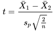
This t test depends on two equations, which are described in Wikipedia. One equation is for a pooled standard deviation, which is the square root of the average variance across the two random samples from the same population. The S_p term references the pooled standard deviation. The sample variance for the members in each sample X₁ and X₂, are simply divided by two to derive the pooled sample variance, which is the average variance across both samples.

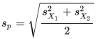
After the pooled standard deviation is computed, you can divide the difference between the means from each sample (X-bar₁ and X-bar₂) by the pooled standard deviation weighted by the number of members (n) in each sample across both samples. The degrees of freedom for the computed t value is 2n - 2 where n is sum of the sample size for each group. Therefore, if the sample size for each group is six, then the degrees of freedom for the computed t value is ten.

These equations were programmed in SQL for the SQL starter statistics package. The starter package includes a stored procedure named compute_t_between_2_groups. The stored procedure implements the preceding two equations. This add-on tip to the starter package embeds the compute_t_between_2_groups stored procedure in a new one named compute_t_between_2_groups_with_lookup. The new stored procedure takes an input parameter designating whether to lookup the computed t value in a critical t values set for a one-tailed test or a two-tailed test.

The following script shows the code for the compute_t_between_2_groups_with_lookup stored procedure. The create procedure statement has an @tail_num input parameter. The code expects this parameter to be 1 for a one-tailed test or 2 for a two-tailed test.

The beginning part of the compute_t_between_2_groups_with_lookup stored procedure sets up for and actually invokes the compute_t_between_2_groups stored procedure. The output from the compute_t_between_2_groups stored procedure is inserted into the #two_group_ouput_base_temp table, which consists of a single row of values that include among other values the computed t and the df for the computed t value.

Then, SQL code inner joins the #two_group_ouput_base_temp table with either the critical table of one-tailed t values (Critical_ts_for_mean_difference_test_1_tail_table) or the critical table of two-tailed values (Critical_ts_for_mean_difference_test_2_tail_table). The inner join matches the two sources on df from the #two_group_ouput_base_temp table and the table of critical t values. The @tail_num input parameter guides the join to the critical t values for a one-tailed or a two-tailed test.

A case statement with output named probability_of_significance returns one of four probability levels for the computed t value. The probability_of_significance values are:

• significant beyond .001
• significant beyond .01
• significant beyond .05
• not significant beyond .05

create procedure compute_t_between_2_groups_with_lookup @tail_num int
as
begin

-- create #two_group_ouput_base_temp
begin try
drop table #two_group_ouput_base_temp
end try
begin catch
print '#two_group_ouput_base_temp not available to drop'
end catch

create table #two_group_ouput_base_temp 
(
 avg_group_1 float
,avg_group_2 float 
,mean_difference float
,computed_t float
,df int
)


-- invoke base compute_t_between_2_groups sp
-- and save output in #two_group_ouput_base_temp
insert into #two_group_ouput_base_temp
exec compute_t_between_2_groups

if @tail_num = 1
	-- join critical t values to outtput from sp (#two_group_ouput_base_temp)
	-- use 1_tailed critical t values
	select  
	 c.avg_group_1
	,c.avg_group_2
	,c.mean_difference
	,c.computed_t
	,t.df
	,case
		when abs(computed_t) > t_001 then 'significant beyond .001 level for one-tailed test'
		when abs(computed_t) > t_01 then 'significant beyond .01 level for one-tailed test'
		when abs(computed_t) > t_05 then 'significant beyond .05 level for one-tailed test'
		else 'not significant beyond .05 level'
	 end probability_of_significance 
	 ,@tail_num [test tail type]
	from #two_group_ouput_base_temp c
	inner join [dbo].[Critical_ts_for_mean_difference_test_1_tail_table] t
	on c.df = t.df
else
	if @tail_num = 2
	-- join critical t values to outtput from sp (#two_group_ouput_base_temp)
	-- use 2_tailed critical t values
	select  
	 top 1 
	 c.avg_group_1
	,c.avg_group_2
	,c.mean_difference
	,c.computed_t
	,t.df
	,case
		when abs(computed_t) > t_001 then 'significant beyond .001 level for two-tailed test'
		when abs(computed_t) > t_01 then 'significant beyond .01 level for two-tailed test'
		when abs(computed_t) > t_05 then 'significant beyond .05 level for two-tailed test'
		else 'not significant beyond .05 level'
	 end probability_of_significance 
	 ,@tail_num [test tail type]
	from #two_group_ouput_base_temp c
	inner join [dbo].[Critical_ts_for_mean_difference_test_2_tail_table] t
	on c.df = t.df


end

go

The next code segment shows the input and output from the compute_t_between_2_groups_with_lookup stored procedure. The steps in the code are as follows.

• A global temporary table named ##temp_group_scores is created to hold the sample values from the two sets of input sample data.
• Next, six values each from the first and second samples are inserted into the global temporary table. Sample identifier values of Group_1 and Group_2 indicate whether a score is from the first or second sample.
• Then, the code invokes the compute_t_between_2_groups_with_lookup stored procedure twice - initially for a one-tailed test and a second time for a two-tailed test.
• Finally, the code displays the source data for the computed t value.

-- prepare data for stored proc

-- create and populate ##temp_group_scores
begin try
drop table ##temp_group_scores
end try
begin catch
print '##temp_group_scores not available to drop'
end catch


create table ##temp_group_scores 
(
 group_id varchar(10)
,score float 
)
go

-- from --http://www.stat.columbia.edu/~martin/W2024/R2.pdf
-- Two-sample t-tests section
insert into ##temp_group_scores values ('Group_1', 91)
insert into ##temp_group_scores values ('Group_1', 87)
insert into ##temp_group_scores values ('Group_1', 99)
insert into ##temp_group_scores values ('Group_1', 77)
insert into ##temp_group_scores values ('Group_1', 88)
insert into ##temp_group_scores values ('Group_1', 91)
insert into ##temp_group_scores values ('Group_2', 101)
insert into ##temp_group_scores values ('Group_2', 110)
insert into ##temp_group_scores values ('Group_2', 103)
insert into ##temp_group_scores values ('Group_2', 93)
insert into ##temp_group_scores values ('Group_2', 99)
insert into ##temp_group_scores values ('Group_2', 104)

-- end of data prep for stored proc

-- invoke compute_t_between_2_groups_with_lookup sp
exec compute_t_between_2_groups_with_lookup @tail_num = 1
exec compute_t_between_2_groups_with_lookup @tail_num = 2

-- show data for t test
select * from ##temp_group_scores

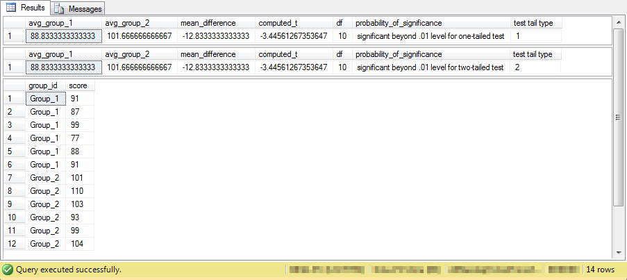
The next screen shot shows the outcome from the preceding script. The first two lines are for the one-tailed test and two-tailed test, respectively. The last twelve lines are for the sample scores from each of two samples. The scores represent reaction times to a stimulus, such as turning on a light. Group 1 is for subjects given a placebo, and Group 2 is for subjects given an active ingredient. The results confirm that the active ingredient slowed reaction times in both a one-tailed test as well as a two-tailed test.

Comparing two sets scores based on different treatments from one sample

Another t test previously addressed in the SQL starter statistics package is one to assess the difference between two sets of measurements on sample members from a single group; this kind of t test is often called a paired sample t test. When using a design for this t test, a data science project reduces sources of variance relative to a two-sample design by re-using the same sample members for two separate rounds of measurements. For example, you could answer the question: is gas mileage better with premium or regular gasoline for a single set of cars? Each car can have its miles per gallon measured twice - once with regular gas and a second time with premium gas.

Like the preceding section, the goal of this section is to develop an adaptation of the starter package code that automatically looks up the statistical significance of a computed t value. Because this type of t test examines two sets of measures for a single group of sample members, it computes a difference between the two measurements for each member. The t test compares the mean size of the differences to the weighted sample standard deviation of the differences between the two sets of measurements.

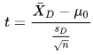
Wikipedia presents the following equation for computing a t value for this kind of test. The X-bar_D term is for the mean of the differences between the measurements for the sample members. The S_D term is for the sample standard deviation of the differences. The number of differences is n, and the reciprocal of the square root of n is the weight for the standard deviation. The degrees of freedom for looking up the statistical significance of the computed t value is n - 1.

The value of mu₀ is frequently omitted, and it is also omitted in this implementation of the test. When the sole goal of the test is just to assess if there is no difference between two sets of measurements, there is no need for a mu₀ term. For this demonstration of the test, we keep a focus on the comparison of two sets of measurements to assess if they are the same or different.

The SQL starter statistics package uses a stored procedure named compute_paired_sample_t for computing this kind of t test. The add-on code re-uses the same stored procedure, but it joins the computed t value and degrees of freedom from the stored procedure to critical t values for either one-tailed or two-tailed tests. The sole advantage of the add-on code for the t test is the automatic lookup of the statistical significance of the computed t value.

The add-on code for the paired sample t test relies on a stored procedure named compute_paired_sample_t_with_lookup. Again, an input parameter named @tail_num allows a user to specify results for either a one-tailed test or a two-tailed test. An If…Else statement facilitates the joining of output from the compute_paired_sample_t stored procedure with one-tailed or two-tailed critical t values. As with the t test from the preceding section, the code reports statistical significance (or its absence) at one of four different levels (not signification at .05, significant at .05, significant at .01, or significant at .001). Here's the code for creating the compute_paired_sample_t_with_lookup stored procedure.

create procedure compute_paired_sample_t_with_lookup @tail_num int
as
begin

-- create #paired_sample_ouput_base_temp
begin try
drop table #paired_sample_ouput_base_temp
end try
begin catch
print '#paired_sample_ouput_base_temp not available to drop'
end catch

create table #paired_sample_ouput_base_temp 
(
 avg_difference float
,computed_t float
,df int
)


-- invoke base compute_paired_sample_t sp
-- and save output in #paired_sample_ouput_base_temp
insert into #paired_sample_ouput_base_temp
exec compute_paired_sample_t


if @tail_num = 1
	-- creates new output column based on probability 
	-- level of significance for one-tailed and two-tailed tests
	select 
	 c.avg_difference
	,c.computed_t
	,c.df
	,case
		when abs(computed_t) > t_001 then 'significant beyond .001 level for one-tailed test'
		when abs(computed_t) > t_01 then 'significant beyond .01 level for one-tailed test'
		when abs(computed_t) > t_05 then 'significant beyond .05 level for one-tailed test'
		else 'not significant beyond .05 level'
	 end probability_of_significance 
	,@tail_num [test tail type] 
	from #paired_sample_ouput_base_temp c
	inner join [dbo].[Critical_ts_for_mean_difference_test_1_tail_table] t
	on c.df = t.df
else
	if @tail_num = 2
	select 
	 c.avg_difference
	,c.computed_t
	,c.df
	,case
		when abs(computed_t) > t_001 then 'significant beyond .001 level for two-tailed test'
		when abs(computed_t) > t_01 then 'significant beyond .01 level for two-tailed test'
		when abs(computed_t) > t_05 then 'significant beyond .05 level for two-tailed test'
		else 'not significant beyond .05 level'
	 end probability_of_significance 
	,@tail_num [test tail type]  
	from #paired_sample_ouput_base_temp c
	inner join [dbo].[Critical_ts_for_mean_difference_test_2_tail_table] t
	on c.df = t.df


end

go

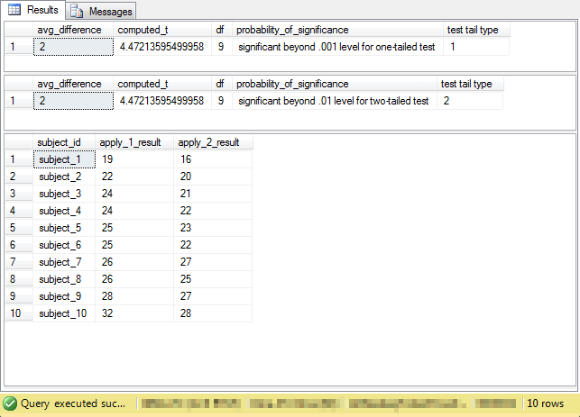
The sample code for this tip also includes a demonstration of the use of the compute_paired_sample_t_with_lookup stored procedure with some sample data. Below is the code for the demonstration; you can view its result sets in following screen shot.

• The ##temp_subject_id_results global temporary table stores the sample data.
• This table has one column for identifying members of each sample data member and two more columns for each set of measurements.
  • The names for first column row entries is arbitrary, but each row should have a unique name. Each of these names should correspond to a single sample member.
  • The names for second and third column row entries are for measurements. This kind of t test requires two measurements for each sample member. In this demonstration, column apply_1_result is for miles per gallon from premium gas and apply_2_result is for miles per gallon from regular gas.
• The output shows the outcome for a one-tailed test followed by a two-tailed test. As you can see, the average difference of two miles per gallon is significant at beyond the .001 level for a one-tailed test, but the same difference is significant at beyond the .01 level for a two-tailed test.
• The final set of output rows show the input data for the computed t values.

-- prepare data for stored proc


-- create and populate ##temp_subject_id_results
begin try
drop table ##temp_subject_id_results
end try
begin catch
print '##temp_subject_id_results not available to drop'
end catch

create table ##temp_subject_id_results
(
 subject_id varchar(10)
,apply_1_result float
,apply_2_result float 
)
go

--delete from ##temp_subject_id_results

-- from --http://www.stat.columbia.edu/~martin/W2024/R2.pdf
-- Paired t-tests section
insert into ##temp_subject_id_results values ('subject_1', 19, 16)
insert into ##temp_subject_id_results values ('subject_2', 22, 20)
insert into ##temp_subject_id_results values ('subject_3', 24, 21)
insert into ##temp_subject_id_results values ('subject_4', 24, 22)
insert into ##temp_subject_id_results values ('subject_5', 25, 23)
insert into ##temp_subject_id_results values ('subject_6', 25, 22)
insert into ##temp_subject_id_results values ('subject_7', 26, 27)
insert into ##temp_subject_id_results values ('subject_8', 26, 25)
insert into ##temp_subject_id_results values ('subject_9', 28, 27)
insert into ##temp_subject_id_results values ('subject_10', 32, 28)

-- end of data prep for stored proc

-- invoke compute_paired_sample_t_with_lookup sp
exec compute_paired_sample_t_with_lookup @tail_num = 1
exec compute_paired_sample_t_with_lookup @tail_num = 2

-- show data for t test
select * from ##temp_subject_id_results

Comparing one set of scores from one sample to a standard value

This is the first section of three in this tip dealing with t tests for which the computed t value is calculated from scratch. In other words, there is a no dependence on a prior tip for this t test.

The t test for this section is unique from other tests in this tip in that it depends on just one sample and just one set of measurements. The computed t value assesses via a two-tailed significance test whether a set of scores for members from a single sample are the same or different from a standard value. You can use a one-tailed version of this test to assess if a set of scores from a sample is greater (or less) than a standard value.

Wikipedia offers the following formula for computing the t value for this kind of test. The test is named the one-sample t test in Wikipedia. As you can see, the equation for this computed t value is very similar to the one in the preceding section for assessing the difference between two sets of measurements from a single sample. The main difference is that this test does not require two sets of measurements for a single sample. In fact, just one set of measurements are required for this test.

The x-bar term is for the mean of the sample scores. The S term is for the sample standard deviation of the scores in the sample. The n term represents the number of scores in the sample. The term mu₀ represents the standard value to which the mean of the sample scores are compared; this term is used in the demonstration for this t test. The degrees of freedom are n - 1 for looking up the statistical significance of the computed t value.

The stored procedure for this t test has the name compute_one_sample_t_with_lookup. This stored procedure takes two input parameter values. The first of these values is for the @tail_num parameter that lets a user specify whether to lookup the statistical significance of the computed t value for a one-tailed test or a two-tailed test. This stored procedure also has an input parameter named @mu_value, which is for the value of mu₀.

The code for creating the stored procedure appears next.

• A pair of queries, one nested within the other, populate the #one_sample_ouput_base_temp table with values for calculating the computed t value.
  • The for_one_sample_computed_t inner query computes the mean, standard deviation, and sample size based on the members in the sample. The input sample scores reside in the ##temp_group_scores global table, which is populated from the code invoking the compute_one_sample_t_with_lookup stored procedure.
  • The outer query populates the #one_sample_ouput_base_temp temporary table with the inherited values, the value of @mu_value, and the computed t value and its degrees of freedom. The @mu_value is included when evaluating the computed t value.
• Next, an If…Else statement facilitates joining the #one_sample_ouput_base_temp table with either one-tailed or two-tailed critical t values for assessing the statistical significance of the computed t value. The @tail_num input parameter determines which set of critical values are used for assessing the statistical significance of the computed t value.
• Statistical significance is evaluated to one of four distinct levels (not significant beyond .05, significant beyond .05, significant beyond .01, or significant beyond .001).

create procedure compute_one_sample_t_with_lookup @tail_num int, @mu_value float
as
begin

declare @mu float = @mu_value


-- create #one_sample_ouput_base_temp
begin try
drop table #one_sample_ouput_base_temp
end try
begin catch
print '#one_sample_ouput_base_temp not available to drop'
end catch

create table #one_sample_ouput_base_temp 
(
 x_bar float
,mu float
,s float
,computed_t float
,df int
)

insert into #one_sample_ouput_base_temp
select 
 x_bar
 ,@mu mu
 ,s
,(x_bar-@mu)/(s/sqrt(n)) computed_t
,df = n - 1
from
(
select 
 avg(score) x_bar
,stdev(score) s
,count(*) n
from ##temp_group_scores
) for_one_sample_computed_t

if @tail_num = 1
		select 
		 x_bar
		,mu
		,s
		,computed_t
		,c.df
		,case
				when abs(computed_t) > t_001 then 'significant beyond .001 level for two-tailed test'
				when abs(computed_t) > t_01 then 'significant beyond .01 level for two-tailed test'
				when abs(computed_t) > t_05 then 'significant beyond .05 level for two-tailed test'
				else 'not significant beyond .05 level'
			 end probability_of_significance
		,@tail_num [test tail type]
 
		from #one_sample_ouput_base_temp c
		inner join [dbo].[Critical_ts_for_mean_difference_test_1_tail_table] t
		on c.df = t.df
else 
	if @tail_num = 2

	select 
	 x_bar
	,mu
	,s
	,computed_t
	,c.df
	,case
			when abs(computed_t) > t_001 then 'significant beyond .001 level for two-tailed test'
			when abs(computed_t) > t_01 then 'significant beyond .01 level for two-tailed test'
			when abs(computed_t) > t_05 then 'significant beyond .05 level for two-tailed test'
			else 'not significant beyond .05 level'
		 end probability_of_significance 
 		,@tail_num [test tail type]

	from #one_sample_ouput_base_temp c
	inner join [dbo].[Critical_ts_for_mean_difference_test_2_tail_table] t
	on c.df = t.df

end

go

The sample data used for demonstrating the computation of the one-sample computed t value is derived from data and a worked example by professor Martin A. Lindquist when he served in the Statistics department at Columbia university. The url for the web resource appears with the sample data and worked example in a comment line within the code below.

• As you can see, the code for invoking the compute_one_sample_t_with_lookup stored procedure follows the same outline as for the preceding three code examples on running the stored procedure for invoking code to compute a t value and lookup its statistical significance.
• The fact that all members contributing data to the computed t value are from a single population is underscored by each row having a group_ID value of Group_1 in the ##temp_group_scores table.
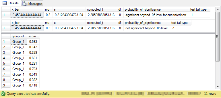
• The @mu_value parameter is .3. In the sample of measurements used for this demonstration, this is the standard salmonella count for ice cream batches that are counted as safe. Salmonella count values greater than .3 are not safe.
• The MPN/g count for a sample of 9 ice cream batches is 0.4564, which is clearly greater than the upper limit for a safe value of .3.
• The null hypothesis tested is whether the MPN/g count less than or equal to .3. Consequently, the alternative hypothesis is whether the MPN/g count is greater than .3.
• Because testing is for greater than a standard value, a one-tailed t test is required.

-- prepare data for stored proc

-- create and populate ##temp_group_scores
begin try
drop table ##temp_group_scores
end try
begin catch
print '##temp_group_scores not available to drop'
end catch

go

create table ##temp_group_scores 
(
 group_id varchar(10)
,score float 
)
go

-- from --http://www.stat.columbia.edu/~martin/W2024/R2.pdf
-- Two-sample t-tests section
insert into ##temp_group_scores values ('Group_1', 0.593)
insert into ##temp_group_scores values ('Group_1', 0.142)
insert into ##temp_group_scores values ('Group_1', 0.329)
insert into ##temp_group_scores values ('Group_1', 0.691)
insert into ##temp_group_scores values ('Group_1', 0.231)
insert into ##temp_group_scores values ('Group_1', 0.793)
insert into ##temp_group_scores values ('Group_1', 0.519)
insert into ##temp_group_scores values ('Group_1', 0.392)
insert into ##temp_group_scores values ('Group_1', 0.418)

-- end of data prep for stored proc

-- invoke stored procedures for one sample t test
exec compute_one_sample_t_with_lookup  @tail_num = 1, @mu_value = .3
exec compute_one_sample_t_with_lookup  @tail_num = 2, @mu_value = .3

-- show data for t test
select * from ##temp_group_scores

The output from the preceding code appears in the following screen shot.

• Results are presented for one-tailed and two-tailed tests, but only the one-tailed test results apply to the hypothesis being tested in this case.
• The results are significant at the .05 probability level for a one-tailed test. This test is the appropriate one for the sample data.
• The counts for individual batches of ice cream appear below the .05 significance level for a two-tailed test. This test is only run to confirm the operation of the code.

Comparing two means from samples with equal or unequal sample sizes and equal variance

Up to this point in the tip, we considered one two-sample t test. Comparing the difference between the means for two independent samples is a common data science requirement. However, there are several slight variations among two-sample t tests.

• The first t test in this tip is for two samples with the same sample size and variance. This is the t test previously demonstrated in the "Comparing two means from samples with the same size" section.
• The t test for this section is for the case where the sample sizes can be different between the two samples, but the variance is assumed to be the same.
• The t test for the next section is for the case where the sample sizes can be different, but the variances are assumed to be different.

I found a couple of highly useful resources for calculating a computed t value for the differences between two sample means with unequal sample sizes (Wikipedia and StatsDirect). The StatsDirect site was particularly helpful because it offered a worked example and helpful intermediate result sets. The code for this section relies on the data from the StatsDirect sample demonstration and the equations for Wikipedia.

The Wikipedia site offers two equations for computing a t value and degrees of freedom when computing a t value between two samples which can have unequal sample sizes.

• The top-level equation is for the computed t value. The two terms X-bar₁ and X-bar₂ refer, respectively, to the means for the first and second samples. The S_p term is for the pooled standard deviation across the two samples. The terms n₁ and n₂ are, respectively, for the sample sizes of the first and second samples.

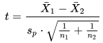
• The equation for the pooled standard deviation appears below. The S²-sub-X₁ term and the S²-sub-X₂ terms are, respectively, the sample variance for the first and second samples. You can use the built-in T-SQL functions for computing the values of these terms.

• The degrees of freedom (df) for looking up the statistical significance of the computed t value is n1 + n2 - 2. This is an implicit equation for the degrees of freedom.

The following script shows the create procedure statement for computing a t value and interpreting it relative to a one-tailed or two-tailed type of t test. This interpretation includes calculating the appropriate degrees of freedom for the sample data that serves as a source for the computed t value and matching those degrees of freedom with corresponding critical t values.

• The name of the stored procedure is compute_t_between_2_groups_with_unequal_sizes_with_lookup.
• The @tail_num input parameter allows a user to designate either a one-tailed or two-tailed comparison.
• An If…Else statement allows one of two blocks of code to execute.
  • Within each code block, the computed t value is calculated and then matched to appropriate critical t values.
  • A case statement assigns a probability level for the computed t value relative to the appropriate critical t values.
  • A collection of nested queries within the If and Else code blocks derives computed t values.
    • The innermost nested subqueries have the names Group_1 and Group_2; these subqueries compute the mean, variance, and sample size within each group.
    • Next, a subquery with a cross join brings the mean, variance, and sample size for each group into a single-line result set for the for_computed_t subquery. In addition, the subquery with the cross join computes the pooled standard deviation and the difference between the means from the two samples.
    • The subquery containing the cross join subquery develops the computed t value and the degrees of freedom for looking up appropriate critical t values.
    • Finally, the outermost query within each If…Else code block computes the probability level of obtaining a computed t value relative to the appropriate critical t values.

create procedure compute_t_between_2_groups_with_unequal_sizes_with_lookup @tail_num int
as
begin

if @tail_num = 1
	select
	 c.avg_group_1
	,c.avg_group_2
	,c.mean_difference
	,c.computed_t
	,c.df
	,case
		when abs(computed_t) > t_001 then 'significant beyond .001 level for one-tailed test'
		when abs(computed_t) > t_01 then 'significant beyond .01 level for one-tailed test'
		when abs(computed_t) > t_05 then 'significant beyond .05 level for one-tailed test'
		else 'not significant beyond .05 level'
	end probability_of_significance 
	,@tail_num [test tail type]
	from
	(
	select
	 mean_Group_1 avg_group_1
	,mean_Group_2 avg_group_2
	,mean_difference
	,mean_difference/t_dnom computed_t
	, (n1-1) + (n2-1) df
	from
	(
	-- Combined results for Group_1 and Group_2
	-- with inputs for computed_t
	select 
	 *
	,sqrt(((n1-1)*variance_Group_1 + (n2-1)*variance_Group_2)/((n1-1)+(n2-1))) sp
	,sqrt(1/cast(n1 as float) + 1/cast(n2 as float)) sp_multiplier
	,sqrt(((n1-1)*variance_Group_1 + (n2-1)*variance_Group_2)/((n1-1)+(n2-1)))
	 *
	 sqrt(1/cast(n1 as float) + 1/cast(n2 as float)) t_dnom
	,(mean_Group_1 - mean_Group_2) mean_difference
	from
	(
	-- Group_1 results
	select 
	 count(*) n1 
	,avg(score) mean_Group_1
	,var(score) variance_Group_1
	from ##temp_group_scores where group_id = 'Group_1'
	) Group_1

	cross join

	(
	-- Group_2 results
	select 
	 count(*) n2 
	,avg(score) mean_Group_2
	,var(score) variance_Group_2
	from ##temp_group_scores where group_id = 'Group_2'
	) Group_2
	) for_computed_t
	) c
	inner join [dbo].[Critical_ts_for_mean_difference_test_1_tail_table] t
	on c.df = t.df
else
	if @tail_num = 2
	select
	 c.avg_group_1
	,c.avg_group_2
	,c.mean_difference
	,c.computed_t
	,c.df
	,case
		when abs(computed_t) > t_001 then 'significant beyond .001 level for two-tailed test'
		when abs(computed_t) > t_01 then 'significant beyond .01 level for two-tailed test'
		when abs(computed_t) > t_05 then 'significant beyond .05 level for two-tailed test'
		else 'not significant beyond .05 level'
	end probability_of_significance 
	,@tail_num [test tail type]
	from
	(
	select
	 mean_Group_1 avg_group_1
	,mean_Group_2 avg_group_2
	,mean_difference
	,mean_difference/t_dnom computed_t
	, (n1-1) + (n2-1) df
	from
	(
	-- Combined results for Group_1 and Group_2
	-- with inputs for computed_t
	select 
	 *
	,sqrt(((n1-1)*variance_Group_1 + (n2-1)*variance_Group_2)/((n1-1)+(n2-1))) sp
	,sqrt(1/cast(n1 as float) + 1/cast(n2 as float)) sp_multiplier
	,sqrt(((n1-1)*variance_Group_1 + (n2-1)*variance_Group_2)/((n1-1)+(n2-1)))
	 *
	 sqrt(1/cast(n1 as float) + 1/cast(n2 as float)) t_dnom
	,(mean_Group_1 - mean_Group_2) mean_difference
	from
	(
	-- Group_1 results
	select 
	 count(*) n1 
	,avg(score) mean_Group_1
	,var(score) variance_Group_1
	from ##temp_group_scores where group_id = 'Group_1'
	) Group_1

	cross join

	(
	-- Group_2 results
	select 
	 count(*) n2 
	,avg(score) mean_Group_2
	,var(score) variance_Group_2
	from ##temp_group_scores where group_id = 'Group_2'
	) Group_2
	) for_computed_t
	) c
	inner join [dbo].[Critical_ts_for_mean_difference_test_2_tail_table] t
	on c.df = t.df
end

go

The next code block shows the SQL for loading sample data into the ##temp_group_scores table. This table holds the data for a computed t value.

• The sample data comes from the StatsDirect web site. The sample is for female rat weights based on a high protein diet versus a low protein diet.
• There is a total of 19 data points:
  • 12 data points for the first group (high protein)
  • 7 additional data points for the second group (low protein)
• Two exec statements run both one-tailed and two-tailed tests for the sample data, but the one-tailed test is the appropriate one for assessing if the high protein diet results in greater weights among the rats than a low protein diet. The two-tailed test is included merely to confirm the operation of the Else block in the If…Else statement for the compute_t_between_2_groups_with_unequal_sizes_with_lookup stored procedure.

-- prepare data for stored proc

-- create and populate ##temp_group_scores
begin try
drop table ##temp_group_scores
end try
begin catch
print '##temp_group_scores not available to drop'
end catch


create table ##temp_group_scores 
(
 group_id varchar(10)
,score float 
)
go

-- from --https://www.statsdirect.co.uk/help/parametric_methods/utt.htm
-- Two-sample t-tests section with unequal sample sizes
insert into ##temp_group_scores values ('Group_1', 134)
insert into ##temp_group_scores values ('Group_1', 146)
insert into ##temp_group_scores values ('Group_1', 104)
insert into ##temp_group_scores values ('Group_1', 119)
insert into ##temp_group_scores values ('Group_1', 124)
insert into ##temp_group_scores values ('Group_1', 161)
insert into ##temp_group_scores values ('Group_1', 107)
insert into ##temp_group_scores values ('Group_1', 83)
insert into ##temp_group_scores values ('Group_1', 113)
insert into ##temp_group_scores values ('Group_1', 129)
insert into ##temp_group_scores values ('Group_1', 97)
insert into ##temp_group_scores values ('Group_1', 123)
insert into ##temp_group_scores values ('Group_2', 70)
insert into ##temp_group_scores values ('Group_2', 118)
insert into ##temp_group_scores values ('Group_2', 101)
insert into ##temp_group_scores values ('Group_2', 85)
insert into ##temp_group_scores values ('Group_2', 107)
insert into ##temp_group_scores values ('Group_2', 132)
insert into ##temp_group_scores values ('Group_2', 94)

-- end of data prep for stored proc

exec compute_t_between_2_groups_with_unequal_sizes_with_lookup @tail_num = 1
exec compute_t_between_2_groups_with_unequal_sizes_with_lookup @tail_num = 2

-- show data for t test
select * from ##temp_group_scores

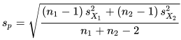
The output from the preceding script appears in following screen shot.

• The results are statistically significant for a one-tailed test at beyond the .05 probability level.
• The two-tailed test outcome is shown to confirm the operation of code for that path in an If…Else block.
• The display of input scores verifies the values used to derive a computed t value.

Comparing two means from samples with unequal variances

When comparing two means where the samples are known (or suspected) to have unequal variances, you can use the t test described in this section. At a top-line conceptual level, there are three equations to consider for the computed t value: the difference between the sample means, the divisor term for the difference between the sample means, and a process for arriving at a degrees of freedom for discovering appropriate critical t values for the t test.

• The first equation is the same as for the t test in the preceding section. It is merely the mean for the first sample less the mean for the second sample.
• The second and third equations are substantially different from the preceding t test, and they are more complicated from a computational perspective.

In addition to Wikipedia, I found a couple of other highly informative references for the t test in this section. Because of the computational complexity of this t test, it is especially useful to have worked examples as references. The Real Statistics Using Excel website had an especially rich explanation of the theory behind this test as well as good coverage of best practices for simplifying the computations for this kind of t test. Adjunct professor Marcus John Hamilton of the University of New Mexico offers a detailed worked example for computing a t test for two samples with unequal variances. This tip uses professor Hamilton's sample data because it was so easy to perform unit tests with the help of his published example, and it allows a cross check of the computing framework from the Real Statistics Using Excel website.

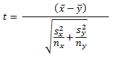
The Real Statistics Using Excel website offers five equations that were coded in SQL within this tip for developing a computed t value and its matching degrees of freedom. The following is the first of the equations for the computed t value. The x-bar term is for the mean of the first sample. The y-bar term is for the mean of the second sample. The S²-sub-X terms and the S²-sub-Y terms are, respectively, the sample variances for the first and second samples. The n_x and n_y terms are, respectively, the number of observations in the first and second samples. The equation below is modified slightly from the original source for this tip to omit unused terms (mu_x and mu_y) in the source web page. This action additionally helps to keep the focus for the example on the difference between group means.

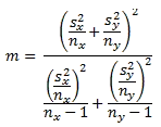
The degrees of freedom for the computed t value is represented by m in the following equation. The other terms in the equation are defined in the preceding equation. Notice that the equation for the degrees of freedom is considerably more elaborate than any of the preceding t tests that do not account for unequal variances between two samples.

Because of the complexity of the above expression, Satterthwaite's correction is widely used for computing the degrees of freedom for the t test. I present three additional equations based on Satterthwaite's correction as described in the website that facilitate the computation of degrees of freedom for samples with unequal variance.

• The degrees of freedom can be represented by following more simple equation. The n terms are defined as above, and the c terms are given in the following two equations.

• The c_x term is specified by the following equation. Again, the S and n terms are defined as in the equation for the computed t value.

• The c_y term is defined, in turn, as one less c_x.

Given these equations for processing a computed t value from two samples with unequal variance, we can use the same general SQL approach for assessing statistical significance as described in the preceding section. The detailed adapted code appears below.

• As you can see, the name of the stored procedure is compute_t_between_2_groups_with_unequal_variances_with_lookup.
• The @tail_num input parameter allows a user to specify either a one-tailed test or a two-tailed test.
• An If…Else statement runs the one-tailed test when the value of @tail_num equals one or the two-tailed test when the value of @tail_num equals two.
• Within the SQL query statement for the If and Else clauses of the If…Else statement are a series of nested subqueries.
  • The innermost subqueries named Group_1 and Group_2 compute the sample mean, variance, and size for each of the two groups.
  • A cross join of the result set for the two innermost subqueries returns a single row with means, variances, and sizes for each of the two groups.
• The c subquery containing the cross joined results computes intermediate values based on the preceding equations for the computed t value and degrees of freedom.
• The outermost query within If and Else code blocks return final results for display from the stored procedure. For example, the outermost query performs a join to select the appropriate critical t values for assessing the statistical significance of the computed t value. The outermost query also uses a case statement to report the probability level for rejecting the null hypothesis or that it is not appropriate to reject the null hypothesis.

create procedure compute_t_between_2_groups_with_unequal_variances_with_lookup @tail_num int
as
begin

if @tail_num = 1
	select 
	 Group_1_mean
	,Group_2_mean
	,mean_difference
	,computed_t
	,c.df
	,case
		when abs(computed_t) > t_001 then 'significant beyond .001 level for one-tailed test'
		when abs(computed_t) > t_01 then 'significant beyond .01 level for one-tailed test'
		when abs(computed_t) > t_05 then 'significant beyond .05 level for one-tailed test'
		else 'not significant beyond .05 level'
	end probability_of_significance 
	,@tail_num [test tail type]
	from
	(
		-- detailed results
		select 
			n1
		,Group_1_mean
		,Group_1_var
		,n2
		,Group_2_mean
		,Group_2_var
		,sqrt((Group_1_var/n1) + (Group_2_var/n2)) t_div
		,(Group_1_mean - Group_2_mean) mean_difference
		,
		-- computation of computed t
		(Group_1_mean - Group_2_mean)
			/
			sqrt((Group_1_var/n1) + (Group_2_var/n2)) computed_t
		,
		-- computation of c for Group_1
		(Group_1_var/n1)/((Group_1_var/n1)+(Group_2_var/n2)) Group_1_c
		,
		-- computation of c for Group_2
		(1-(Group_1_var/n1)/((Group_1_var/n1)+(Group_2_var/n2))) Group_2_c
		,round(((n1-1)*(n2-1))
			/
			(
			(n1-1)*power((1-(Group_1_var/n1)/((Group_1_var/n1)+(Group_2_var/n2))),2)
			+(n2-1)*power((Group_1_var/n1)/((Group_1_var/n1)+(Group_2_var/n2)),2)
			),0) df
		from
		(
		select 
			count(*) n1
		,avg(score) Group_1_mean
		,var(score) Group_1_var
		from ##temp_group_scores where group_id = 'Group_1'
		) summary_Group_1

		cross join

		(
		select 
			count(*) n2
		,avg(score) Group_2_mean
		,var(score) Group_2_var
		from ##temp_group_scores where group_id = 'Group_2'
		) summary_Group_2
	)c
	inner join [dbo].[Critical_ts_for_mean_difference_test_1_tail_table] t
	on c.df = t.df

else
	if @tail_num = 2
	select 
	 Group_1_mean
	,Group_2_mean
	,mean_difference
	,computed_t
	,c.df
	,case
		when abs(computed_t) > t_001 then 'significant beyond .001 level for two-tailed test'
		when abs(computed_t) > t_01 then 'significant beyond .01 level for two-tailed test'
		when abs(computed_t) > t_05 then 'significant beyond .05 level for two-tailed test'
		else 'not significant beyond .05 level'
	end probability_of_significance 
	,@tail_num [test tail type]
	from
	(
		-- detailed results
		select 
			n1
		,Group_1_mean
		,Group_1_var
		,n2
		,Group_2_mean
		,Group_2_var
		,sqrt((Group_1_var/n1) + (Group_2_var/n2)) t_div
		,(Group_1_mean - Group_2_mean) mean_difference
		,
		-- computation of computed t
		(Group_1_mean - Group_2_mean)
			/
			sqrt((Group_1_var/n1) + (Group_2_var/n2)) computed_t
		,
		-- computation of c for Group_1
		(Group_1_var/n1)/((Group_1_var/n1)+(Group_2_var/n2)) Group_1_c
		,
		-- computation of c for Group_2
		(1-(Group_1_var/n1)/((Group_1_var/n1)+(Group_2_var/n2))) Group_2_c
		,round(((n1-1)*(n2-1))
			/
			(
			(n1-1)*power((1-(Group_1_var/n1)/((Group_1_var/n1)+(Group_2_var/n2))),2)
			+(n2-1)*power((Group_1_var/n1)/((Group_1_var/n1)+(Group_2_var/n2)),2)
			),0) df
		from
		(
		select 
			count(*) n1
		,avg(score) Group_1_mean
		,var(score) Group_1_var
		from ##temp_group_scores where group_id = 'Group_1'
		) summary_Group_1

		cross join

		(
		select 
			count(*) n2
		,avg(score) Group_2_mean
		,var(score) Group_2_var
		from ##temp_group_scores where group_id = 'Group_2'
		) summary_Group_2
	)c
	inner join [dbo].[Critical_ts_for_mean_difference_test_2_tail_table] t
	on c.df = t.df

end

go

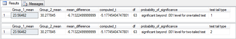
The next two screen shots show the results from the one-tailed test and the two-tailed test. Both tests yield results that are statistically significant at beyond the .001 level. The data represent the thickness in centimeters of two different decorative styles of ceramic sherds from an archaeological site. As you can see, the sample means are substantially different; this corresponds to the outcome of the t tests. There are 25 ceramic sherd measurements for the first group and 40 sherd measurements for the second group. You cannot directly see a comparison of the variances of the two groups, but that will be covered in the next section.

Are the variances from two samples unequal?

One of two t tests can apply to two-sample data when samples have unequal sizes.

• If the two samples also have unequal variances, then apply the t test from the preceding section.
• If two samples have unequal sample sizes, but their population variances cannot be verified to be significantly different, then apply the t test from the section just before the preceding section.

However, it may not be perfectly obvious just from examining data points from two samples when two samples come from populations with unequal variances. There are a couple of statistical tests for comparing the variances between two samples. This tip illustrates the use of the F test for the ratio of the variances between two samples.

The NIST/SEMATECH e-Handbook of Statistical Methods presents a general discussion along with sample data for using the F test to assess if the variances of two populations from which two samples come are equal. If the variances from two samples are unequal enough to suggest that they come from populations with different variances, the F values at df_num and df_dnom degrees of freedom for the ratio of the two variances will be distributed in one of two critical F distribution regions. This concept is more fully explained in the "Computing and saving lookup tables containing critical values" section and the next paragraph.

An F distribution has two degrees of freedom - one for the left tail and a second one for the right tail. When comparing the ratio of the variances for two samples, the ratios are distributed as an F distribution. If sample size for the numerator of the ratio is n₁, then the degrees of freedom for the numerator is n₁ - 1. If sample size for the denominator of the ratio is n₂, then the degrees of freedom for the denominator is n₂ - 1. You can lookup the F distribution for the F distribution's two tails from the Critical_Fs_for_variance_test_table object described in the "Computing and saving lookup tables containing critical values" section.

The following script presents a create procedure statement for assessing if the ratio of the variances is statistically significant at beyond the .05 probability level, which is the level used for the Critical_Fs_for_variance_test_table object with a two-tailed test. As you can see, a collection of nested queries resides within the procedure.

• The procedure's name is compute_F_between_2_groups_for_variances_with_lookup.
• The group_1_var and group_2_var subqueries compute the variances for the first and second samples, respectively. These subqueries also compute sample sizes and degrees of freedom for the first and second samples.
• A cross join query between the two innermost subqueries combines the results from the first and second groups into a single row. Additionally, the subquery with the cross join computes the ratio of the variances between the two groups.
• The outermost query joins the result set from the subquery with the cross join to the Critical_Fs_for_variance_test_table object. A case statement in the outermost query assigns a value of 'significant at beyond .05' or 'not significant at beyond .05' to the are_variances_different column based on the ratio of the variances.

create procedure compute_F_between_2_groups_for_variances_with_lookup
as
begin

select 
 c.var_Group_1
,c.df_Group_1
,c.var_Group_2
,c.df_Group_2
,c.F
,
case
	when (var_Group_1/var_Group_2) < f.[left-tail-f] 
		or (var_Group_1/var_Group_2) > f.[right-tail-f] 
		then 'significant at beyond .05'
		else 'not significant at beyond .05'
end [are_variances_different]
from
(
select 
 var_Group_1
,df_Group_1
,var_Group_2
,df_Group_2
,var_Group_1/var_Group_2 F
from
(
select 
 group_id
,var(score) var_Group_1
,count(*) n_Group_1
,count(*)-1 df_Group_1
from ##temp_group_scores
where group_id = 'Group_1'
group by group_id
) group_1_var

cross join

(
select 
 group_id
,var(score) var_Group_2 
,count(*) n_Group_2
,count(*)-1 df_Group_2
from ##temp_group_scores
where group_id = 'Group_2'
group by group_id
) group_2_var
) c
inner join [dbo].[Critical_Fs_for_variance_test_table] f
on c.df_Group_1 = f.df_num
and c.df_Group_2 = f.df_dnom

end

go

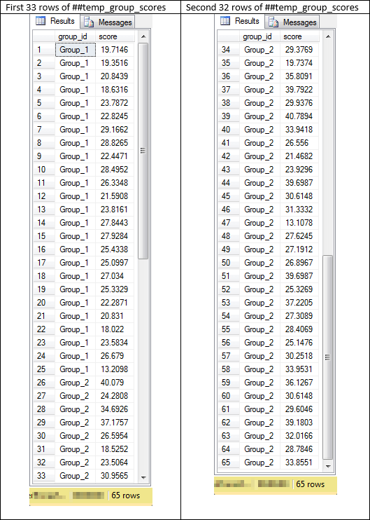
The following script shows the application of the compute_F_between_2_groups_for_variances_with_lookup stored procedure to the data from the "Comparing two means from samples with unequal variances" section.

• The script initially creates an empty copy of the ##temp_group_scores table.
• Then, it uses a set of insert statements to pump the sample data points from the "Comparing two means from samples with unequal variances" section into the table.
• Finally, it invokes the compute_F_between_2_groups_for_variances_with_lookup stored procedure to compute the F value and assess if it is statistically significant.

-- create and populate ##temp_group_scores
begin try
drop table ##temp_group_scores
end try
begin catch
print '##temp_group_scores not available to drop'
end catch


create table ##temp_group_scores 
(
 group_id varchar(10)
,score float 
)
go

-- from --https://www.unm.edu/~marcusj/2Sampletex2.pdf
-- Two-sample t-tests section with unequal sample variances
insert into ##temp_group_scores values ('Group_1', 19.7146)
insert into ##temp_group_scores values ('Group_1', 19.3516)
insert into ##temp_group_scores values ('Group_1', 20.8439)
insert into ##temp_group_scores values ('Group_1', 18.6316)
insert into ##temp_group_scores values ('Group_1', 23.7872)
insert into ##temp_group_scores values ('Group_1', 22.8245)
insert into ##temp_group_scores values ('Group_1', 29.1662)
insert into ##temp_group_scores values ('Group_1', 28.8265)
insert into ##temp_group_scores values ('Group_1', 22.4471)
insert into ##temp_group_scores values ('Group_1', 28.4952)
insert into ##temp_group_scores values ('Group_1', 26.3348)
insert into ##temp_group_scores values ('Group_1', 21.5908)
insert into ##temp_group_scores values ('Group_1', 23.8161)
insert into ##temp_group_scores values ('Group_1', 27.8443)
insert into ##temp_group_scores values ('Group_1', 27.9284)
insert into ##temp_group_scores values ('Group_1', 25.4338)
insert into ##temp_group_scores values ('Group_1', 25.0997)
insert into ##temp_group_scores values ('Group_1', 27.034)
insert into ##temp_group_scores values ('Group_1', 25.3329)
insert into ##temp_group_scores values ('Group_1', 22.2871)
insert into ##temp_group_scores values ('Group_1', 20.831)
insert into ##temp_group_scores values ('Group_1', 18.022)
insert into ##temp_group_scores values ('Group_1', 23.5834)
insert into ##temp_group_scores values ('Group_1', 26.679)
insert into ##temp_group_scores values ('Group_1', 13.2098)
insert into ##temp_group_scores values ('Group_2', 40.079)
insert into ##temp_group_scores values ('Group_2', 24.2808)
insert into ##temp_group_scores values ('Group_2', 34.6926)
insert into ##temp_group_scores values ('Group_2', 37.1757)
insert into ##temp_group_scores values ('Group_2', 26.5954)
insert into ##temp_group_scores values ('Group_2', 18.5252)
insert into ##temp_group_scores values ('Group_2', 23.5064)
insert into ##temp_group_scores values ('Group_2', 30.9565)
insert into ##temp_group_scores values ('Group_2', 29.3769)
insert into ##temp_group_scores values ('Group_2', 19.7374)
insert into ##temp_group_scores values ('Group_2', 35.8091)
insert into ##temp_group_scores values ('Group_2', 39.7922)
insert into ##temp_group_scores values ('Group_2', 29.9376)
insert into ##temp_group_scores values ('Group_2', 40.7894)
insert into ##temp_group_scores values ('Group_2', 33.9418)
insert into ##temp_group_scores values ('Group_2', 26.556)
insert into ##temp_group_scores values ('Group_2', 21.4682)
insert into ##temp_group_scores values ('Group_2', 23.9296)
insert into ##temp_group_scores values ('Group_2', 39.6987)
insert into ##temp_group_scores values ('Group_2', 30.6148)
insert into ##temp_group_scores values ('Group_2', 31.3332)
insert into ##temp_group_scores values ('Group_2', 13.1078)
insert into ##temp_group_scores values ('Group_2', 27.6245)
insert into ##temp_group_scores values ('Group_2', 27.1912)
insert into ##temp_group_scores values ('Group_2', 26.8967)
insert into ##temp_group_scores values ('Group_2', 39.6987)
insert into ##temp_group_scores values ('Group_2', 25.3269)
insert into ##temp_group_scores values ('Group_2', 37.2205)
insert into ##temp_group_scores values ('Group_2', 27.3089)
insert into ##temp_group_scores values ('Group_2', 28.4069)
insert into ##temp_group_scores values ('Group_2', 25.1476)
insert into ##temp_group_scores values ('Group_2', 30.2518)
insert into ##temp_group_scores values ('Group_2', 33.9531)
insert into ##temp_group_scores values ('Group_2', 36.1267)
insert into ##temp_group_scores values ('Group_2', 30.6148)
insert into ##temp_group_scores values ('Group_2', 29.6046)
insert into ##temp_group_scores values ('Group_2', 39.1803)
insert into ##temp_group_scores values ('Group_2', 32.0166)
insert into ##temp_group_scores values ('Group_2', 28.7846)
insert into ##temp_group_scores values ('Group_2', 33.8551)

exec compute_F_between_2_groups_for_variances_with_lookup

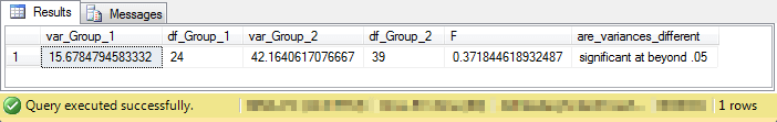
Here's a screen shot with output from the preceding script.

• Recall that the sample sizes for the first and second groups are, respectively, twenty-five and forty. Therefore, the corresponding degrees of freedom are twenty-four and thirty-nine.
• As you can see, the variances are significantly different, which is the a priori assumption for the data in the "Comparing two means from samples with unequal variances" section.

The next script shows the application of the compute_F_between_2_groups_for_variances_with_lookup stored procedure to the data in the "Comparing two means from samples with equal or unequal sample sizes and equal variance" section. The data for this section had unequal sample sizes of twelve and seven for the first and second samples, respectively.

• The code starts by truncating the ##temp_group_scores table initially created and populated above.
• Next, a sequence of insert statements populates the table with data from the "Comparing two means from samples with equal or unequal sample sizes and equal variance" section.
• Finally, the compute_F_between_2_groups_for_variances_with_lookup stored procedure is invoked.

truncate table ##temp_group_scores

-- from --https://www.statsdirect.co.uk/help/parametric_methods/utt.htm
-- Two-sample t-tests section with unequal sample sizes
insert into ##temp_group_scores values ('Group_1', 134)
insert into ##temp_group_scores values ('Group_1', 146)
insert into ##temp_group_scores values ('Group_1', 104)
insert into ##temp_group_scores values ('Group_1', 119)
insert into ##temp_group_scores values ('Group_1', 124)
insert into ##temp_group_scores values ('Group_1', 161)
insert into ##temp_group_scores values ('Group_1', 107)
insert into ##temp_group_scores values ('Group_1', 83)
insert into ##temp_group_scores values ('Group_1', 113)
insert into ##temp_group_scores values ('Group_1', 129)
insert into ##temp_group_scores values ('Group_1', 97)
insert into ##temp_group_scores values ('Group_1', 123)
insert into ##temp_group_scores values ('Group_2', 70)
insert into ##temp_group_scores values ('Group_2', 118)
insert into ##temp_group_scores values ('Group_2', 101)
insert into ##temp_group_scores values ('Group_2', 85)
insert into ##temp_group_scores values ('Group_2', 107)
insert into ##temp_group_scores values ('Group_2', 132)
insert into ##temp_group_scores values ('Group_2', 94)

-- end of data prep for stored proc

exec compute_F_between_2_groups_for_variances_with_lookup

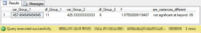
Here's a screen shot with the results from the preceding section. As the name of the section implies, the sample variances are not significantly different from each other at the .05 probability level.

Next Steps

Try the stored procedures and scripts for loading and running with your own data. If you encounter difficulties review the content in the remainder of this section.

All the sample scripts for this tip were run from the AllNasdaqTickerPricesfrom2014into2017 database with two new tables copied from two Excel worksheet files. You can download the file with the SQL scripts and the worksheet files from here.

If you want to run code for the first two t tests demonstrated in this tip, then you will also need to download the initial version of the SQL statistics package because two stored procedures are referenced in this tip from that release of the package.

While all code testing was performed for the AllNasdaqTickerPricesfrom2014into2017 database, you do not strictly need that database. You do, however, need the relevant script files and the SQL Server tables based on the worksheet files. The worksheet files and the SQL scripts are available for download from this tip. If you want, you can download the AllNasdaqTickerPricesfrom2014into2017 database from here.

About the author

Rick Dobson is an author and an individual trader. He is also a SQL Server professional with decades of T-SQL experience that includes authoring books, running a national seminar practice, working for businesses on finance and healthcare development projects, and serving as a regular contributor to MSSQLTips.com. He has been growing his Python skills for more than the past half decade -- especially for data visualization and ETL tasks with JSON and CSV files. His most recent professional passions include financial time series data and analyses, AI models, and statistics. He believes the proper application of these skills can help traders and investors to make more profitable decisions.

This author pledges the content of this article is based on professional experience and not AI generated.

View all my tips