By: Rick Dobson | Updated: 2024-03-20 | Comments (2) | Related: > TSQL
Problem
I am a Microsoft SQL Server database developer assigned to support a team of data scientists. I need help understanding how to compute with T-SQL and interpret the mode of dataset values. Please present some sample code and commentary to get me started computing the mode in data science projects.
Solution
The mode is one of a trilogy of central tendency indicators for the values in a dataset. The purpose of a central tendency indicator is to return one (or more) values that represent central or typical values in a dataset. A prior MSSQLTips.com article provides a good overview of exploratory data analysis, including the mean, median, and mode central tendency indicators. MSSQLTips.com also published another tip that illustrates how to compute a mode, but it processed only a few small datasets. One more tip drills down on a use case and code samples for arithmetic means, geometric means, and medians; this tip used a relatively small sample size.
This SQL tutorial revisits the topic of calculating modes in T-SQL from data in a SQL database. Special emphasis is given to computing source datasets via Python on which to calculate modes. By controlling the source dataset programmatically, you can illustrate special features of modes, such as how to calculate modes for multimodal distributions. This tip bases its datasets on normal distributions, but the approach illustrated in this tip can be extended to accommodate other distribution types, such as lognormal, Poisson, exponential, binomial, and uniform distributions.
What is a Mode for a Dataset?
The mode for a dataset is a discrete value with the largest count or a binned collection of continuous values with the largest relative frequency count. A dataset can have 0, 1, or 2+ modes. For datasets based on symmetrically distributed data, it is common to discover 1 mode per dataset. In this case, the modal value is the single dataset value with the largest relative frequency or count of discrete values in a dataset. For example, for a dataset with just six values like these (1, 2, 3, 3, 4, 5), the mode is 3. The mode is 3 because its count is greater than any other dataset value.
A dataset derived from a multimodal distribution can have two or more values with the largest count. This is an example of a dataset with two modes: 1, 2, 3, 3, 4, 5, 6, 7, 8, 8, 9, 10. The two modal values are 3 and 8. Each of these dataset values has a count of two, which is larger than the count for any other dataset values.
It is also possible for a dataset not to have a mode. This can occur when all the discrete values in the dataset occur with equal frequency. In this case, no dataset value is more common than any other dataset value.
Given the above examples, it is easy to derive how to compute a mode. Count the frequency for each discrete dataset value or the relative frequency within each bin of continuous dataset values. Return one or more modal values; these modal values are the largest counts for the discrete values or the largest relative frequencies for bins of continuous values in the source data.
A Normal Frequency Distribution with Mean = 100 and Standard Deviation = 15
A normal frequency distribution in data analysis is an example of a unimodal distribution with a bell-shaped curve of dataset value counts. The count at the top of the bell-shaped curve defines a single modal value. A normal distribution in statistics derives from a probability density function. The normal distribution depends on the mean and standard deviation of the values within the distribution. When the mean is 0 and the standard deviation is 1, the distribution is called a standard normal distribution or a z distribution.
The numpy library for Python has a built-in function named normal for returning randomly distributed normal values. The following Python script shows how to use the normal function to create a million random normal deviate values with a mean of 100 and a standard deviation of 15. The numpy normal function populates an array of float values. The code subsequently transforms the float values to integer values in a pandas dataframe, which are stored in a CSV file named normal_data_100_15_1000000.csv. The one million normal deviates in the df dataframe are binned, counted and displayed as a histogram by the plt application programming interface in the matplotlib library.
# prepared by Rick Dobson for MSSQLTips.com

import numpy as np
from numpy.random import seed
from numpy.random import normal
import pandas as pd
import matplotlib.pyplot as plt

# make this example reproducible
seed(1)

# generate sample of 1000000 values
# that follow a normal distribution
data = normal(loc=100, scale=15, size=1000000)

#print (data)

# save the NumPy array to a Python list
list_1 = data.tolist()

# convert the Python list to a pandas dataframe (df)
# with int datatype values and no column header
# print the df

df = pd.DataFrame(list_1)
df = df.astype('int')
print(df)

# save df to normal_data_100_15_1000000.csv
df.to_csv('normal_data_100_15_1000000.csv', header=False, index=False)

# aggregate normal deviate values to bins(20)
# then show the histogram
count, bins, ignored = plt.hist(df, 20)
plt.title('normal_data_100_15_1000000\n\n')
plt.show()
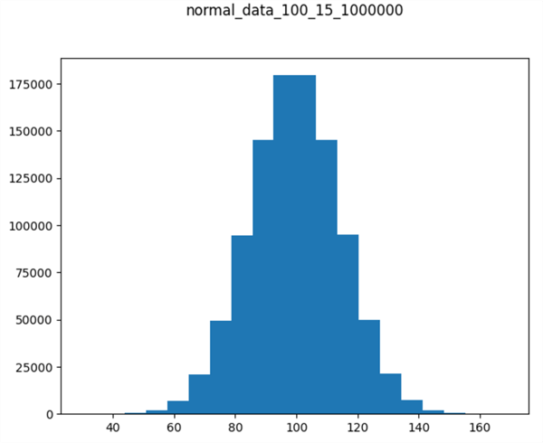
Here's the histogram displayed by the preceding script. The title denotes the chart is for 1000000 normally distributed values with a mean of 100 and a standard deviation of 15. Dataset values appear along the x-axis, and counts appear along the y-axis. Notice that the histogram chart appears to be approximately bell-shaped.

Reading a CSV File of Dataset Values into a SQL Server Table to Compute a Mode
The T-SQL script in this section reads with the bulk insert statement the values from the normal_data_100_15_1000000.csv file into a SQL Server table named normal_data_100_15_1000000. A subsequent nested select statement finds and displays the dataset value from the normal_data_100_15_1000000 table with the largest frequency count. Here is the syntax:
-- prepared by Rick Dobson for MSSQLTips.com

-- specify DataScience as the default database
use DataScience
go

-- create a fresh table to store
-- 1000000 normal deviates from Python

drop table if exists [dbo].[normal_data_100_15_1000000]

create table normal_data_100_15_1000000 (
normal_deviate int)

-- populate the normal_data_100_15_1000000 table
-- in the dbo schema of the default database
-- from normal_data_100_15_1000000.csv file
bulk insert [dbo].[normal_data_100_15_1000000]
from  'C:\my_py_scripts\normal_data_100_15_1000000.csv'
with ( format = 'CSV');

-- compute mode value for unimodal normal_deviate
-- distribution with the largest count
select [normal_deviate] [mode]
from
(
-- select normal_deviate with the largest count
select top 1 [normal_deviate] [normal_deviate], count(*) [deviate count]
from [DataScience].[dbo].[normal_data_100_15_1000000]
group by [normal_deviate]
order by [deviate count] desc
) to_compute_mode
The following screenshot shows the results set returned by the nested select statement in the preceding script. The modal normal_deviate value is 99 with a count of 26653.
The normal deviate values were examined further in an Excel spreadsheet (not shown here) to verify the results, and the outcome below appears valid and reasonable.
- The range of normal_deviate values starts with an integer value of 30 and extends through a maximum value of 169.
- No normal_deviate value had a larger count than the count for the dataset value of 99. Therefore, this integer is the modal integer value for the dataset.
- The fiftieth percentile normal_deviate value, commonly referred to as the median, was between 99 and 100.
- The arithmetic average of the normal_deviate values is 99.53676471.
Recall that the normal_deviate values returned by the numpy normal function are continuous float values and not discrete integer values. The float values returned by the normal function were converted to Integer values with the astype method; this conversion introduces a slight distortion from the originally returned float values to their nearest matching integer values. Furthermore, any collection of numpy normal function return values is a random sample from a huge range of possible normal values. Taking a different sample based on another seed value or an internally specified seed value can result in a different set of normal_deviate values from the explicitly specified seed value of 1 in the preceding Python script.

A Normal Frequency Distribution with Mean = 200 and Standard Deviation = 15
This section presents a Python script for creating a normal frequency distribution with a mean of 200 and a standard deviation of 15. The new normal frequency distribution is saved in a CSV file named 'normal_data_200_15_1000000.csv'.
As you can see, the script is nearly identical to the script in the "A normal frequency distribution with mean = 100 and standard deviation = 15" section. The major difference besides the CSV file name changing is a new parameter value for the loc parameter in the normal function. The loc parameter in this section is 200, but the loc parameter for the script in the earlier section, creating a normal distribution, is 100. The loc parameter in the numpy normal function specifies the mean of the normal deviate values returned by the function.
It is also important that the seed parameter value is 1 for the script in this section and in the earlier section, creating a normal distribution. The seed parameter specifies the return normal deviate values from a known starting value. Because of designating a known starting value, the normal distribution is reproducible in successive runs of the script. Additionally, the scale parameter value is the same for the scripts in both sections. This means that both distributions have the same standard deviation value. Since the standard deviation controls the shape of a normal distribution, the shapes of the two distributions are the same.
# prepared by Rick Dobson for MSSQLTips.com

import numpy as np
from numpy.random import seed
from numpy.random import normal
import pandas as pd
import matplotlib.pyplot as plt

# make this example reproducible
seed(1)

# generate sample of 1000000 values
# that follow a normal distribution
data = normal(loc=200, scale=15, size=1000000)

#print (data)

# save the NumPy array to a Python list
list_1 = data.tolist()

# convert the Python list to a pandas dataframe (df)
# with int datatype values and no column header
# print the df

df = pd.DataFrame(list_1)
df = df.astype('int')
print(df)

# save df to normal_data_200_15_1000000.csv
df.to_csv('normal_data_200_15_1000000.csv', header=False, index=False)

# aggregate normal deviate values to bins(20)
# then show the histogram
count, bins, ignored = plt.hist(df, 20)
plt.title('normal_data_200_15_1000000\n\n')
plt.show()
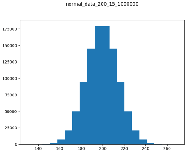
The following chart shows a histogram populated with the normal values returned by the preceding script. There are two key points to note. First, the histogram is bell-shaped. Second, the x values along the horizontal axis are about 100 units greater than in the preceding normal distribution. Therefore, by concatenating the normal deviate values from the previously created normal distribution with the normal deviate values from the script in this section, we can create a bimodal distribution. The next section shows how to accomplish this with some T-SQL code.

Creating and Processing a Bimodal Distribution with T-SQL
This final section of the current tip walks you through an example for computing modes with T-SQL queries across two concatenated sets of normal deviate values.
- The first step in the example is to concatenate two sets of normal deviate values into a single SQL Server table. This step uses bulk insert statements to transfer the normal deviate values in the normal_data_100_15_1000000.csv and the normal_data_200_15_1000000.csv files into SQL Server tables named after each of the two CSV files.
- The second step has three actions within it.
- First, it concatenates the normal_data_100_15_1000000 table and the normal_data_200_15_1000000 table into a new fresh temp table named #temp_unioned_normal_deviate_sets. Within the context of the current tip, the #temp_unioned_normal_deviate_sets table has two million normal deviate values.
- Next, the second step processes the #temp_unioned_normal_deviate_sets table by unique normal_deviate values so that each row in the new table (#temp_normal_deviate_counts) contains unique normal_deviate values along with their counts. For the data in this tip, the number of rows in the #temp_normal_deviate_counts table declines to 236 rows from the two million rows in the #temp_unioned_normal_deviate_sets table.
- The third action is to compute a value for a local variable named @mode_count. This local variable is the count for one or more normal_deviate values with the largest counts from the #temp_normal_deviate_counts table.
- The third step filters the table of normal_deviate values with their counts in the #temp_normal_deviate_counts table to find rows with [deviate count] values equal to @mode_count. These rows correspond to modal values in the original #temp_unioned_normal_deviate_sets table.
-- prepared by Rick Dobson for MSSQLTips.com

-- specify DataScience as the default database
use DataScience
go

declare @mode_count bigint

-- create a fresh table to store
-- 1000000 normal deviates from Python

drop table if exists [dbo].[normal_data_100_15_1000000]

create table normal_data_100_15_1000000 (
normal_deviate int)

-- populate the normal_data_100_15_1000000 table
-- in the dbo schema of the default database
-- from normal_data_100_15_1000000.csv file
bulk insert [dbo].[normal_data_100_15_1000000]
from  'C:\my_py_scripts\normal_data_100_15_1000000.csv'
with ( format = 'CSV');

-- create a fresh table to store
-- 1000000 normal deviates from Python

drop table if exists [dbo].[normal_data_200_15_1000000]

create table normal_data_200_15_1000000 (
normal_deviate int)

-- populate the normal_data_200_15_1000000 table
-- in the dbo schema of the default database
-- from normal_data_200_15_1000000.csv file
bulk insert [dbo].[normal_data_200_15_1000000]
from  'C:\my_py_scripts\normal_data_200_15_1000000.csv'
with ( format = 'CSV');

--------------------------------------------------------------------

-- compute a fresh unioned set of deviate values and populate

--  concatenate two normal deviate sets

drop table if exists #temp_unioned_normal_deviate_sets

select *
into #temp_unioned_normal_deviate_sets
from [dbo].[normal_data_100_15_1000000]

union all

select * from [dbo].[normal_data_200_15_1000000]

-- populate #temp_normal_deviate_counts
-- and compute @mode_count

drop table if exists #temp_normal_deviate_counts

select normal_deviate, count(*) [deviate count]
into #temp_normal_deviate_counts
from #temp_unioned_normal_deviate_sets
group by normal_deviate

-- optionally display column values in #temp_normal_deviate_counts
-- select * from #temp_normal_deviate_counts

set @mode_count = (
select top 1 [deviate count]
from #temp_normal_deviate_counts
order by [deviate count] desc)

-- optionally display @mode_count
-- select @mode_count

--------------------------------------------------------------------

-- extract modal values from #temp_normal_deviate_counts
-- these are the modes for the concatenated distribution
select *
from #temp_normal_deviate_counts
where [deviate count] = @mode_count
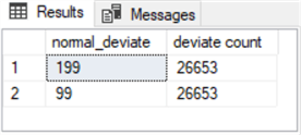
Here is the results set from the preceding script.
- There are two modal values in the results set.
- The normal_data_100_15_1000000 table contributes a modal value of 99.
- The normal_data_200_15_1000000 table contributes a modal value of 199.
- Both modes have a deviate count value of 26653.

Next Steps
This tip introduces the basics of what is a mode and how to compute modes for relatively large samples with 1,000,000 or 2,000,000 dataset values. Python generates underlying dataset values and stores the values in CSV files. The tip also shows how to read the CSV files from Python with a T-SQL script. A T-SQL script is also used to combine data from two different CSV files. The use case for combining CSV files in T-SQL also allows you to compute modes for multimodal distributions.
Download the sample dataset files.
There are several next steps for extending this tip depending on your needs.
- First, you can compare the mode as a measure of central tendency versus the arithmetic mean and the median for unimodal distributions, such as a normal distribution.
- Second, you can compare the mode versus other central tendency indicators when working with multimodal distributions. If the underlying data are truly multimodal, the multiple modes may easily create a more valid representation of typical values than an arithmetic mean or a median.
- Third, you can create datasets having more than two modes. This extension may have special value for cases where it is useful to model production data coming from different factories at alternative geographic locales.
- If underlying data are highly skewed, such as for income distribution in a country, then modal values may be much better at discovering typical values than arithmetic means, which tend to be heavily influenced by outlier values.
About the author
 Rick Dobson is an author and an individual trader. He is also a SQL Server professional with decades of T-SQL experience that includes authoring books, running a national seminar practice, working for businesses on finance and healthcare development projects, and serving as a regular contributor to MSSQLTips.com. He has been growing his Python skills for more than the past half decade -- especially for data visualization and ETL tasks with JSON and CSV files. His most recent professional passions include financial time series data and analyses, AI models, and statistics. He believes the proper application of these skills can help traders and investors to make more profitable decisions.
This author pledges the content of this article is based on professional experience and not AI generated.
View all my tips
Article Last Updated: 2024-03-20


