Problem
I support a data science team that often asks for datasets with different distribution values in uniform, normal, or lognormal shapes. Please present and demonstrate the T-SQL code for populating datasets with random values from each distribution type. I also seek graphical and statistical techniques for assessing how a random sample corresponds to a distribution type.
Solution
Data science projects can require processing and simulation of all kinds of data. Three of these kinds of data are briefly referenced below.
- Uniform Value Distribution: Sometimes, a data science project may require the creation of sample datasets where each of several items occurs an approximately equal number of times. For example, a lottery can require winning lottery numbers from uniformly distributed data—that is, every possible lottery number has an equal chance of winning.
- Normal Value Distribution: Other times, a data science project may need data that are normally distributed where values occur most commonly for a central value, such as a mean, and the relative frequency of values declines in a symmetric way the farther away they are from a central value. This kind of distribution is common for the IQ scores or the heights of students at a school.
- Lognormal Value Distribution: Another type of distribution sometimes used in data science projects is one where values are skewed to the right. A lognormal function is one kind of distribution that exhibits this tendency. In a lognormal distribution, there are relatively many values near the lower end of a distribution of values, and the relative frequency of values declines sharply for larger values. The distribution of personal incomes or the population of cities in a collection of cities can have this type of distribution.
This tip presents and describes the T-SQL code for generating the preceding three distribution types. You will also be exposed to quantitative as well as graphical techniques for verifying the distribution of values in a dataset.
Generating and Verifying Uniform Value Distributions
The main objective of this tip section is to illustrate how to generate a set of random integer values that are uniformly distributed – that is, whose frequencies of occurrence are about the same for all integers.
- The Microsoft documentation for SQL Server reveals that the T-SQL rand() function returns pseudo-random float values from 0 through 1, exclusive. Float values returned by the rand() function can be transformed to integers by an expression that depends on the minimum and maximum integer values as well as a floor() function.
- This section also demonstrates how to program a Chi Square goodness of fit test to assess statistically how well the rand() function and floor function work together to return uniformly distributed integer values. The statistical test draws on values that can be returned by the CHISQ.INV.RT() function in Excel. If you decide to use another approach for generating uniformly distributed random integers besides the one demonstrated in this tip, you should consider using the statistical test to ensure that your alternative approach also satisfies the requirement of uniformity across a range of integer values.
- The section closes with a histogram chart for the results set from a T-SQL select statement for the output from the process described in this section. You can use the histogram to visually assess how uniformly the integers are distributed.
The following script shows a T-SQL script for generating the random integers as well as implementing the Chi Square test to assess if the random integers are uniformly distributed across a designated set of values. The script also shows the outcome of copying a T-SQL results set into Excel for creating a histogram.
The script has four sections; each section is separated from the preceding one by a line of comment markers.
The first section starts with a use statement to designate a default database (DataScience); you can use any other database you prefer.
- The @min_integer and @max_integer local variables allow you to designate the range of integer values in your results set of random integer values.
- The @loop_ctr and @max_loop_ctr local variables are for controlling the number of uniform random integers generated.
- The @number_of_integers local variable is for storing the count of integer values that are randomly generated.
The second section is to create a table for storing the random integer values (#rand_integers). The rows of the table are populated with the rand() function inside a while loop. The loop populates the #rand_integers table with @max_loop_ctr random integer values. At the conclusion of this section, the uniform random numbers are generated. The next two sections are for helping you to verify by either a statistical test or a histogram chart if the generated values are uniformly distributed.
MSSQLTips.com previously published a tip for introducing the rand() function to T-SQL developers. One of the readers of that tip left a comment with his preferred approach that he believes is sufficiently faster to use in place of the approach demonstrated in this tip and the earlier one. I do not believe that while loops are an inherently evil approach – especially for dashing off a solution that is quick to code and easy for many beginners T-SQL developers to understand. If you adapt the commenter’s approach you should consider running some assessment of the uniformity of the values generated as well as its performance in comparison to the solution illustrated below.
use DataScience
go

-- This code sample returns a uniform random distribution of
-- digits from @min_integer (1) through @max_integer (10)

-- declare min and max random integer values
-- and compute number of integers in a set
-- echo assigned/computed local variable values
-- set up to generate 100 uniform random digits for a distribution

declare
 @min_integer tinyint =   1
,@max_integer tinyint =  10
,@number_of_integers tinyint
,@loop_ctr int = 0
,@max_loop_ctr int = 100

set @number_of_integers = (@max_integer - @min_integer) + 1

select
 @max_loop_ctr [@max_loop_ctr]
,@max_integer [@max_integer]
,@min_integer [@min_integer]
,@number_of_integers [@number_of_integers]

--------------------------------------------------------------------------

-- create a fresh copy of #rand_integers
drop table if exists #rand_integers

create table #rand_integers
(
rand_integer tinyint
)

-- loop @max_loop_ctr times
while @loop_ctr < @max_loop_ctr
begin

-- generate a random digit from @min_integer through @max_integer
-- and insert it into #rand_integers
insert #rand_integers(rand_integer)
select floor(rand()*(@max_integer - @min_integer + 1) + @min_integer)

set @loop_ctr = @loop_ctr + 1

end

--------------------------------------------------------------------------

-- assess the goodness of fit
-- to a uniform distribution

-- create a fresh copy of #ChiSquareCriticalValues
-- the critical values are for a distribution test
drop table if exists #ChiSquareCriticalValues
create table #ChiSquareCriticalValues
(
 [df/prob.] tinyint null
,[.05] float null
,[.01] float null
,[.001] float null
)

-- bulk insert forChiSquareCriticalValues.cs file
-- to #ChiSquareCriticalValues
bulk insert #ChiSquareCriticalValues
from 'C:\My Text Files for SQL Server\forChiSquareCriticalValues.csv'
with (
 format = 'CSV'
,firstrow = 2
,fieldterminator = ','
)
--,rowterminator = '0x0a')

select * from #ChiSquareCriticalValues

--------------------------------------------------------------------------

-- compute, save, and display chi_square_component for each integer
drop table if exists #chi_square_components

select
 for_chi_square.rand_integer
,for_chi_square.frequency
,for_chi_square.[expected frequency]
,power((for_chi_square.frequency - for_chi_square.[expected frequency]),2)
 /for_chi_square.[expected frequency] [chi_square component]
 into #chi_square_components
from
(
-- compute frequency and expected frequency values for each integer
select
rand_integer
,count(*) [frequency]
,cast(@max_loop_ctr as real)/cast(@number_of_integers as real) [expected frequency]
from #rand_integers
group by rand_integer
) for_chi_square
order by for_chi_square.rand_integer

select *  from #chi_square_components

-- Compare Chi Square test statistic to
-- Critical Chi Square value at .05 probability level
select
 sum([chi_square component]) [Chi Square test statistic]
,@number_of_integers-1 [degrees of freedom]
,(select [.05] from #ChiSquareCriticalValues
   where [df/prob.] = (@number_of_integers-1))
  [Critical Chi Square for at least the .05 probability level]
,
 (case
  when sum([chi_square component]) <
    (select [.05] from #ChiSquareCriticalValues
   where [df/prob.] = (@number_of_integers-1))  then 'it is a uniform distribution'
   else 'it is not a uniform distribution'
  end) [test result]
from #chi_square_components
The last two sections in the preceding code segment illustrate how to run a Chi Square goodness-of-fit test. This test depends on the CHISQ.INV.RT function from within Excel. The following screenshot excerpt shows critical Chi Square goodness-of-fit values for degrees of freedom from 1 through 30 for significance levels of .05, .01, and .001. For those who want more in-depth coverage from MSSQLTips.com of the Chi Square goodness-of-fit test, you are referred to this prior tip.

You can copy the values from the spreadsheet content to a CSV file so the critical Chi Square values appear as below. This CSV file is saved at C:\My Text Files for SQL Server\forChiSquareCriticalValues.csv for use by the preceding script.
df/prob.,0.05,0.01,0.001
1,3.841458821,6.634896601,10.82756617
2,5.991464547,9.210340372,13.81551056
3,7.814727903,11.34486673,16.2662362
4,9.487729037,13.27670414,18.46682695
5,11.07049769,15.08627247,20.51500565
6,12.59158724,16.81189383,22.45774448
7,14.06714045,18.47530691,24.32188635
8,15.50731306,20.09023503,26.12448156
9,16.9189776,21.66599433,27.87716487
10,18.30703805,23.20925116,29.58829845
11,19.67513757,24.72497031,31.26413362
12,21.02606982,26.21696731,32.90949041
13,22.36203249,27.68824961,34.52817897
14,23.6847913,29.14123774,36.12327368
15,24.99579014,30.57791417,37.69729822
16,26.2962276,31.99992691,39.25235479
17,27.58711164,33.40866361,40.79021671
18,28.86929943,34.80530573,42.31239633
19,30.14352721,36.19086913,43.82019596
20,31.41043284,37.56623479,45.31474662
21,32.67057334,38.93217268,46.79703804
22,33.92443847,40.28936044,48.26794229
23,35.17246163,41.63839812,49.72823247
24,36.4150285,42.97982014,51.17859778
25,37.65248413,44.3141049,52.61965578
26,38.88513866,45.64168267,54.05196239
27,40.11327207,46.96294212,55.47602021
28,41.33713815,48.27823577,56.89228539
29,42.5569678,49.58788447,58.30117349
30,43.77297183,50.89218131,59.7030643
The third section in the preceding script uses a bulk insert statement to copy the critical Chi Square values to the SQL Server #ChiSquareCriticalValues table. The third section also displays a results set with the frequency (count) for each integer instance saved in the second script section. The fourth section of the preceding script computes the Chi Square test value and compares the test value to the values in the #ChiSquareCriticalValues table.
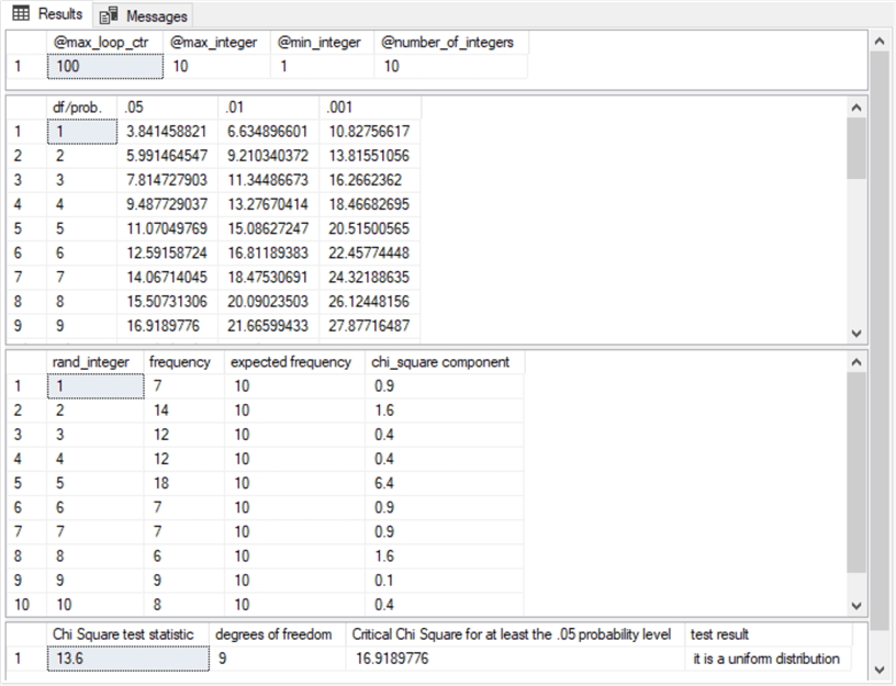
The following screenshot shows the beginning row(s) of the four results sets from the preceding script.
- The first results set shows the values assigned to or computed for @max_loop_ctr, @max_integer, @min_integer, and @number_of_integers.
- The second results set displays an excerpt with the first nine rows from the #ChiSquareCriticalValues table. The ninth row in the second column of this table has a value of 16.9189776, which is the critical Chi Square value for statistical significance at .05 with nine degrees of freedom.
- A computed Chi Square value less than this critical value means that the randomly generated values are uniformly distributed.
- A computed Chi Square value greater than or equal to the critical Chi Square value means that the randomly generated values are not uniformly distributed.
- The third results set displays frequency, expected frequency, and Chi Square component value for each of the ten integer values used in this tip’s demonstration.
- The fourth results set displays the results of the statistical goodness-of-fit test.
- The Chi Square test statistic is the sum of the Chi Square component values in the third results set.
- The degrees of freedom is equal to one less than the number of integers, which is 9 in this example.
- The critical Chi Square value for at least the .05 probability level is 16.9189776. Notice that this value matches the value in the ninth row of the second column in the second results set.
- The test result is a text field that indicates the distribution of frequency values does not differ significantly from a uniform distribution.
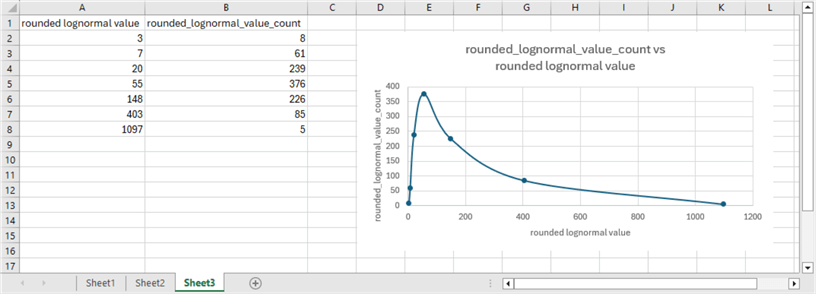
The final screenshot for this section shows the result of copying the rand_integer and frequency column values from third results set to an Excel workbook. The workbook includes chart settings for displaying the frequency of each rand_integer value in a histogram with a column for each rand_integer value.

Generating and Displaying Normal Value Distributions
The normal distribution is among the most popular distributions for data science projects. Many kinds of data are normally distributed, and it is therefore useful to be able to create normally distributed datasets for analysis and simulation objectives. Dallas Snider authored a tip on populating with T-SQL datasets of normally distributed random values based on the Box-Muller transform. According to Wikipedia, this transform converts pairs of uniformly distributed values to normally distributed values. Snider’s implementation of the transform shows how to use SQL Server’s rand() function output to create normally distributed value sets.
The normal distribution values in this tip section are different from the uniform distribution values in the preceding section in several key respects.
- Normally distributed values have a bell-shaped frequency count by normal deviate value. Uniformly distributed values have a rectangular-shaped frequency count by uniform deviate value.
- The frequency counts for normally distributed values near the mean are greater than those farther away from the mean. The frequency counts for uniformly distributed values are generally the same, no matter how close or far away they are from the mean.
This tip section briefly describes a slightly updated version of the original T-SQL code included in the Snider tip on generating normally distributed values. This tip also offers fresh comments about the code to help you derive your own normally distributed datasets. The section concludes with a couple of histogram charts shown in Excel for two different parameter sets to control the shape of a normally distributed value set.
The script below has four sections for deriving normally distributed values.
- The first section starts by designating a default database (Database), but you can name any other database you prefer. Next, a fresh version of the ##tblNormalDistribution table is created. The first section concludes by declaring and populating a set of local variables (from @pi through @precision). The initial assignments for the local variables are:
- @iteration is set equal to 0.
- @pi is set equal to pi().
- @2pi is set equal to 2.0 times @pi.
- @mean and @stdDev are set to 0 and 1, respectively, for the set of normal deviates that you are generating because the code is for normal deviates from a standardized normal distribution. If your target distribution is not a standardized normal distribution, then you can use other values besides 0 and 1 for initializing @mean and @stdDev.
- @precision is the number of spaces to the right of the decimal point for computed normal deviate values.
- @numberOfIterations is the number of iterations that generate normally distributed values. The initial setting of 500 returns 1000 normal deviate values – two normal deviates for each iteration.
- The second section includes a while loop for transforming 1000 uniform deviates into 1000 normal deviates. Two uniform deviates are transformed to normal deviates and inserted into the ##tblNormalDistribution table on each pass through the while loop.
- The third section computes and displays selected statistics on the contents of the ##tblNormalDistribution table after the while loop in the second section concludes.
- The fourth section bins the values for display as a histogram in Excel. Each successive run of the following script can generate a different set of random normal deviates. Furthermore, modifying the initial values for local variables can also change the generated normal deviates in predictable ways.
-- adapted from SQL Server T-SQL Code to Generate A Normal Distribution
-- in MSSQLTips.com

Use DataScience
go

-- creating a temporary table for normal deviates
drop table if exists ##tblNormalDistribution
create table ##tblNormalDistribution (x float)
go

-- declare and set variables
declare @pi float, @2pi float, @randNum1 float, @randNum2 float
declare @value1 float, @value2 float
declare @iteration int, @numberOfIterations int
declare @mean float
declare @stdDev float --standard deviation
declare @precision int --number of places to the right of the decimal point

select @iteration = 0
select @pi = pi()
select @2pi = 2.0 * @pi
select @mean = 0   -- specifies the mean for a normal distribution
select @stdDev = 1 -- specifies the standard deviation for a normal distribution
select @precision = 1
select @numberOfIterations = 500

---------------------------------------------------------------------------------

-- loop for number of iterations
-- each loop generates two random normal deviates
-- in x column of ##tblNormalDistribution
while (@iteration < @numberOfIterations)
begin
  select @randNum1 = rand()
  select @randNum2 = rand()
  select @value1 = round((sqrt(-2.0*log(@randNum1))*cos(@2pi*@randNum2))*@stdDev, @precision)+@mean
  select @value2 = round((sqrt(-2.0*log(@randNum1))*sin(@2pi*@randNum2))*@stdDev, @precision)+@mean

  insert into ##tblNormalDistribution (x) values (@value1)
  insert into ##tblNormalDistribution (x) values (@value2)

  select @iteration = @iteration + 1
end

---------------------------------------------------------------------------------

-- generate statistics for random normal deviates
select count(*) as [Count],
       min(x)   as [Min],
       max(x)   as [Max],
       avg(x)   as [Average],
       stdev(x) as [Standard Deviation] from ##tblNormalDistribution

---------------------------------------------------------------------------------

-- binned normal deviates for a histogram
select round(x,0) as testValue,
count(*) as testValueCount
from ##tblNormalDistribution
group by round(x,0)
order by testValue
The following screenshot shows two histograms of normal deviation values by frequency counts.
- The top histogram is for a standard normal distribution with a mean of 0 and a standard deviation of 1. The values along the horizontal axis are expressed in standard deviation units.
- The second histogram is for an ordinary normal distribution with a mean of 0 and a standard deviation of 1.5. This histogram also shows horizontal coordinates in standard deviation units.
- Notice that the bottom histogram has more testValues along the x-axis than the top histogram. Also, the top histogram is taller than the bottom histogram, with a noticeably larger frequency at its central bin than the bottom histogram. Both outcomes are the result of initializing @stdDev to 1.5 in the bottom histogram versus 1 in the top histogram.

Generating and Displaying Lognormal Value Distributions
This section adapts techniques presented in previous sections for the uniform and normal distributions for generating and displaying a value set with a lognormal distribution. According to Brilliant.org and Wikipedia, the probability density for a lognormal variate is defined by the following equation:
X = eµ+σZ
Where
X is the lognormal probability distribution value
µ is the mean of the logarithm of X
σ is the standard deviation of the logarithm of X
Z is the standard normal variable with a mean of 0 and a standard deviation of 1
If you take the log of both sides of the preceding equation, it may help to clarify why the preceding characterizes the values in a lognormal distribution. The form of the equation after taking the log of both sides changes to:
Log X = µ + σZ
Because Z is a standard normal variate value, log X is also normally distributed. The distribution of log X values has a mean of µ, and its standard deviation is σ. Thus, µ designates the horizontal axis value, and σ controls the shape of the relative frequency or probability density for log X values.
At the end of this section, you will see that a lognormal distribution for X values is especially well suited for describing the distribution of values with a right skew. This is because the X values are the antilog of the lognormal values. The log X values are normally distributed and thus symmetric, but the X values are stretched to the right by positive values of σ. The greater the value of σ, the greater the skew.
Because lognormal values are derived from the log of normally distributed values, the lognormal values must be positive real number values. However, it is common for normally distributed values to display the relative frequency of both positive and negative underlying values. Examine, for example, the two normal distributions charted at the end of the preceding section. Therefore, when computing lognormal values from an underlying normal distribution with negative and/or zero values, it is desirable to transform the distribution of values to the right so that the transformed values start at a value greater than 0.
The following code is designed to transform the normal distributions from the preceding equation with negative, zero, or positive values to only positive values for use in this section. The transformation returns only positive values as input to the log function for the underlying X values.
The code has two sections separated by a row of comment markers.
- The first section computes values for @min and @relo local variables.
- @min is the minimum value in the underlying distribution of normal values. As noted above, it is possible for @min to be a negative or a zero value as well as a positive value.
- @relo is the number of units to move normal values to the right on the horizontal axis.
- Defining @relo_value as abs(@min) + 1 ensures that adding @relo_value to all the underlying normal horizontal distribution values results in a collection of normal horizontal values that are all positive with the same shape parameter (σ) as the original underlying values.
- The second section performs three roles
- It commences by adding @relo_value to all x values in the original normal distribution.
- Next, it calculates e raised to the (x + @relo_value) power.
- The results from these two steps are saved in a fresh copy of the #forlognormals table.
- Next, the transformed x values are rounded to zero places after the decimal before grouping and counting the transformed x values, which are just lognormal values.
- After the second section is completed, the final results set is copied to an Excel spreadsheet for charting and displaying the lognormal values.
use DataScience
go

--find min(x) in ##tblNormalDistribution
declare
 @min float = (select min(x) from ##tblNormalDistribution);

-- declare and assign relocation value (@relo_value)
-- for x in ##tblNormalDistribution
-- transformed x values are moved @relo_value units
-- to the right on the x axis


declare @relo_value float
set @relo_value = abs(@min) + 1

-- display @min and @relo values based on ##tblNormalDistribution
select @min [@min], @relo_value [@relo_value]

----------------------------------------------------------------------

-- relocate x values in ##tblNormalDistribution
-- by @relo units to the right so that
-- all the transformed x values are positive
-- this allows all transformed x values to have log values (log (x))
-- the antilog value of log (x), which is derived,
-- with the exp function, is the lognormal value
select
 x
,@min [@min]
,@relo_value [@relo_value]
,x + @relo_value [transformed x value]
,exp(x + @relo_value) [lognormal value for transformed x value]  -- antilog of log(x)
from ##tblNormalDistribution order by x


-- save [transformed x value] and [lognormal value for transformed x value]
-- in #forlognormals
drop table if exists #forlognormals
select
 x + @relo_value [transformed x value]
,exp(x + @relo_value) [lognormal value for transformed x value]  -- antilog of log(x)
into #forlognormals
from ##tblNormalDistribution order by x

-- display [rounded lognormal value] along with [rounded_lognormal_value_count]
-- round to zero places after the decimal
select round([lognormal value for transformed x value],0) [rounded lognormal value]
 ,count(*) [rounded_lognormal_value_count]
from #forlognormals
group by round([lognormal value for transformed x value],0)
order by round([lognormal value for transformed x value],0)
Here is the relative frequency chart of the lognormal values. The chart appears as a scattergram of the counts for the lognormal values on the vertical axis with lognormal values on the horizontal axis. A curved line connects the points in the scattergram. The scattergram with a curved line connecting the points makes it easy to visualize the skew to the right for the lognormal values. Also, notice that the rounded_lognormal_value counts in the following chart data correspond to the test value counts in the first chart for the normally distributed values in the “Generating and Displaying Normal Value Distributions” section.
Next Steps
This tip introduces the basics of computing distribution function values for three different distribution types –function values that are uniformly, normally, and lognormally distributed. These three distribution types have different functional forms for displaying frequency counts relative to their corresponding distribution values. The computation of frequency counts for each distribution count is based on T-SQL code in SQL Server scripts.
You can assess the correspondence between a set of values in a dataset and a known distribution shape by charting in Excel the frequency counts for functional values. You can adapt the three examples in this tip to your own datasets to verify how well the values in your datasets match any of the three distributions reviewed in this tip. This tip’s download includes an Excel workbook file with a separate workbook tab for each distribution type.
Instead of a visual evaluation for the shape of the values in a dataset, you can use a Chi Square goodness of fit test for actual frequency counts versus expected frequency counts. This approach can yield a precise statistical test result with a probability of getting the test value. This tip implemented the Chi Square goodness of fit test for uniformly distributed values. The same general approach can be adapted to either of the other two distributions examined in this tip.

Rick Dobson is a SQL Server professional with decades of T-SQL experience that includes authoring books, running a national seminar practice, working for businesses on finance and healthcare development projects, and serving as a regular contributor to MSSQLTips.com. He has been a practicing Python developer for more than the past half decade – with a special emphasis for data visualization and ETL tasks with JSON and CSV files. His most recent professional passions include financial time series data and analyses, AI models, and statistics. If you are interested in growing your skills in any of these areas especially as they relate to financial securities, consider visiting his blog at https://securitytradinganalytics.blogspot.com/2023/12/.
- MSSQLTips Awards: Leadership (200+ tips) – 2025 | Author of the Year Contender – 2017-2024