Problem
The fictional company named Adventure Works Cycle [1] always boosts sales with a Spring marketing campaign. This year, marketing managers think of possible changes in customers. For example, managers are concerned that the average annual income of all prospective customers increases to more than $50,000, and the proportion of house owners in all potential customers is not 60% anymore. If either of these two concerns is plausible, they need to improve on last year’s marketing strategies and techniques. Similar situations often occur in the business world, and these business users demand a method to examine their concerns. Because of physical constraints, economic constraints, time constraints, or other constraints, it is usually impractical to verify the truth of such hypotheses directly. How can IT professionals help these business users evaluate the credibility of these hypotheses by a statistical approach?
Solution
We employ statistical hypothesis testing to discover more in-depth insights into our data. We can sample from a population and then reject some preconceived hypotheses based on sample statistics. To perform hypothesis testing for the fictional company, I install the Microsoft sample database AdventureWorksDW2017 [1], in which the database table “ProspectiveBuyer” contains a list of 2,059 prospective customers. I assume that the company cannot obtain data in columns “YearlyIncome” and “HouseOwnerFlag” for all potential customers. Nevertheless, through a survey, the company can collect these data from randomly selected customers.
To have a sample, I randomly select 35 prospective customers from the table. For a small number of customers, the company can collect information for columns “YearlyIncome” and “HouseOwnerFlag.” Then, I walk through the process of hypothesis testing to determine whether these sample statistics provide enough evidence to reject some hypotheses about the population. Generally, statistical hypothesis testing consists of these five steps [2]:
- State the null and alternative hypotheses;
- Compute the test statistic;
- Compute the (1-α) confidence interval for the test statistic;
- State the statistical conclusion;
- Compute p-value;
The use of statistical hypothesis testing provides a powerful tool for decision making [3]. It is worth noting that statistical tests should never constitute the sole input to inferences or decisions about associations or effects [4]. Larry [5] also warned that there was a tendency to use hypothesis testing methods even when they are not appropriate. He recommended that estimation and confidence intervals are better tools.
I organized this tutorial as follows. In Section 1, we explore several elements involved in statistical hypothesis testing: null hypothesis, alternative hypothesis, p-value, test statistic, and so on. Section 2 performs a statistical hypothesis test of a mean. I conduct a statistical hypothesis test of a proportion in Section 3. Next, in Section 4, I list several commonly used hypothesis tests and recommend some further reading materials.
I tested code used in this tip with Microsoft Visual Studio Community 2017 and Microsoft R Client 3.5.2 on Windows 10 Home 10.0 <X64>. The DBMS is Microsoft SQL Server 2017 Enterprise Edition (64-bit).
1 – Elements of Statistical Hypothesis Testing
Doren [6] claimed: “Of all the kinds of knowledge that the West has given to the world, the most valuable is a method of acquiring new knowledge. Called ‘scientific method,’ it was invented by a series of European thinkers from about 1550 to 1700.” Forming a hypothesis and testing it with an experiment is the key difference between the scientific method and other ways of acquiring knowledge [7].
Dr. Helmenstine demonstrated a 6-step procedure of the scientific method [7]. The process starts with formulating general research questions, then conducting some background research, and after that, stating a hypothesis. Next, researchers design an experiment. Researchers perform statistical hypothesis testing to determine whether they should reject the explicit hypothesis based on some samples. The last step is to report the overall conclusions. This procedure involves several elements of statistical hypothesis testing.
1.1 Null Hypothesis and Alternative Hypothesis
Anatole France said, “The greatest virtue of man is perhaps curiosity.” Curiosity is a strong desire to know or learn something. Filled with interests, people ask questions and seek answers. When we observe human behavior or natural phenomena, we may find some associations or effects, and then we ask questions. A sample question is whether red-light cameras installed in a traffic intersection affect the number of vehicle collisions in that intersection [8]. In the business world, we usually have some concerns about situations as well. Here are three examples, and in this exercise, we evaluate the credibility of the last two concerns:
- The cameras affect vehicle collisions.
- The average annual income for Adventure Works Cycles prospective customers is higher than $50,000;
- The proportion of house owners in all Adventure Works Cycles potential customers is not 60%;
We may not be able to develop a measure to assess these concerns directly. However, we can evaluate the logical opposite of these concerns. When a hypothesis is plausible, we can reject its opposite. The following three statements present these opposites of the three concerns mentioned above:
- The cameras installed in traffic intersections did not affect vehicle collisions;
- The average annual income for Adventure Works Cycles prospective customers is less than or equal to $50,000;
- The proportion of house owners in all Adventure Works Cycles potential customers is 60%;
We refer to any logical opposite as a null hypothesis, denoted by H0. The null hypothesis, reflecting the status quo, states how the value of a population parameter used to be or currently is – this is to say, there is no difference or no change. We hope to reject the null hypothesis [9] so that we can further investigate the effect. The alternative hypothesis, denoted by H1, is counter to the null hypothesis and is a statement that we want to support [11]. We write these hypotheses in symbolic notation:
where ![]() is the difference of population means in the occurrence of vehicle collisions before and after the camera installation,
is the difference of population means in the occurrence of vehicle collisions before and after the camera installation, ![]() is the mean of annual income for all prospective customers, and
is the mean of annual income for all prospective customers, and ![]() is the proportion of all potential customers who own a house.
is the proportion of all potential customers who own a house.
In the first hypothesis, we want to compare the means of two populations. In the second hypothesis, we want to compare the mean value of a single group to a hypothesized value. We face different situations when performing statistical hypothesis testing. Several types of hypothesis testing are available for use:
One-sample Test: Studies one population;
Paired Two-Sample Test: Compares a treatment group to a control group when there is a natural one-to-one pairing between the subjects in these two groups.
Independent Two-sample Test: Compares two populations when there is not a natural one-to-one pairing in them. Therefore, two random samples need to be selected from these two populations, respectively.
1.2 Test Statistic
A test statistic is a random variable derived from a sample. We use the value of a test statistic to measure the effect of interest to users and then to draw a statistical conclusion. When interpreting the testing result, someone may conclude to accept the null hypothesis. As a rule, we cannot accept the null hypothesis. Instead, we should say, “fail to reject the null hypothesis” [11].
Every type of hypothesis test has a method for calculating the test statistic. In this exercise, we perform statistical hypothesis testing for population means and proportions. We use the normal distributions or the t-distributions to compute the test statistic. The standard deviation of the population distribution is usually unknown, and we use a sample standard deviation to estimate the population standard deviation. Table 1 gives some examples of test statistic calculation formulas:
| Type | Test Statistic | Assumption | Case | Formula |
|---|---|---|---|---|
| Z-Test | Z-Score | Sample size n is greater than 30. | Single Mean |  |
| Single Proportion | | |||
| T-Test | T-Score | Population distribution is approximately normal. | Single Mean |  |
| Single Proportion | |
Table 1 Some test statistic calculations
The formulas in Table 1 indicate that a test statistic is the transformation of a sample statistic. For example, when a sample statistic, the mean, has a distribution ![]() , the test statistic has the distribution
, the test statistic has the distribution![]() .
.
1.3 Type I and Type II Errors
The statistical hypothesis testing allows us to test a belief about a population by using a sample. The sample may provide sufficient evidence to reject a null hypothesis. On the contrary, we cannot reject a null hypothesis because of insufficient evidence. Whenever we decide, it is always possible that we make a mistake. There are four ways of testing a null hypothesis: two of them lead to correct decisions, and the other two go wrong. We further classify the way that causes a wrong decision into two types: type I error and type II error.
Here are two ways leading to correct decisions:
- The null hypothesis is true, and we do not reject it;
- The null hypothesis is false, and we reject it;
There are two ways of making wrong decisions:
- The null hypothesis is true, and we reject it (type I error);
- The null hypothesis is false, and we fail to reject it (type II error);
A type I error occurs when we reject a true null hypothesis. The probability of making this kind of error, denoted by α, has other names: the level of significance and the significance level. Before we make an inference, we need to determine an acceptable error rate, represented by the significance level. In the business world, many factors, such as company policies, industry standards, and user experience, determine significance levels. The most frequently chosen values of α are 0.10, 0.05, 0.02, and 0.01; their corresponding significance levels are 10%, 5%, 2% and 1% [9].
A type II error occurs when we fail to reject a false null hypothesis. The probability of making this kind of error, denoted by β, depends on several factors, including the type I error rate α, the sample size, and the hypothesis. Book [3] provides calculations and further discussion of β.
When we struggle to avoid rejecting true hypotheses, we are likely to fail to reject false hypotheses. When we decrease the chance of making one type of error, the possibility of making the other type rises. The risk associated with a type I error has traditionally been considered the more serious of the two types of error [9]. For this reason, I use the type I error in this tip.
Inspired by Smith’s explanation [10], Figure 1 illustrates the relation between α and β. The null distribution represents the probability distribution of the test statistic when the null hypothesis is true; the alternative distribution describes the probability distribution of the test statistic when the alternative hypothesis is true. A type I error arises when we do not think that these test statistics in the red area in Figure 1 have the null distribution, but they do. A type II error occurs when we believe these test statistics in the magenta area have the null distribution, but they do not.
When we increase the critical value (i.e., move the dotted line toward the right side), we reject less and, therefore decrease type I error. However, the range of test statistics illustrated by the magenta area increases; consequently, the type II error increases. In a nutshell, moving the critical value to the right decreases the type I error α and increases the type II error β. When we shift the position of the critical value to the left, the value of α increases, and the value of β decreases.
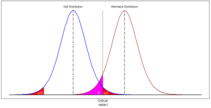
Figure 1 The relation between α and β
Table 2 summarizes four possible outcomes in the hypothesis testing process and their associated probabilities.
| Decision about null hypothesis | Null hypothesis is true | Null hypothesis is false |
| Do not reject the null hypothesis | Correct decision Probability = 1- α | Type II error Probability = β |
| Reject the null hypothesis | Type I error Probability = α | Correct decision Probability = 1- β |
Table 2 Relations between truth and falseness of the null hypothesis
1.4 Rejection Region
Researchers usually want to reject the null hypothesis to show that the effect of interest reflects a real difference [2]. We could erroneously reject a true null hypothesis; the probability of making this error, the type I error, is α. Let’s look at the null hypothesis given in Section 1.1: the cameras installed in traffic intersections did not influence vehicle collisions. We write this hypothesis in symbolic notation:
The report [8] provides crash data before and after installing red-light cameras at 13 intersections. We assume that the distribution of vehicle crash rates is approximately normal. Since the sample size is less than 30, and the standard deviation is unknown, the sample mean has a t-distribution with 12 degrees of freedom. Figure 2 illustrates the shape of the t-distribution with 12 degrees of freedom.
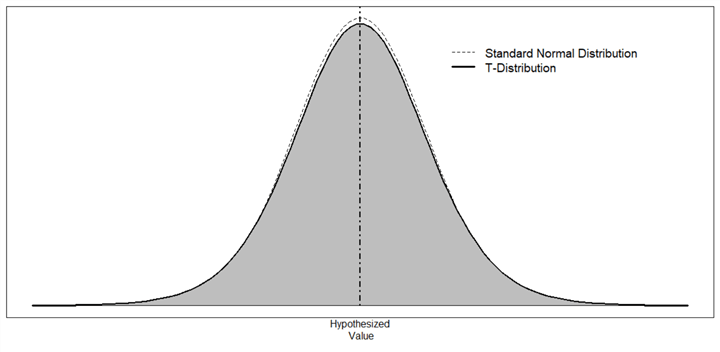
Figure 2 The t-distribution with 12 degrees of freedom
In certain extreme situations, we believe in the status quo, and we neglect any difference, change, or effect revealed in samples. Therefore, we do not reject the null hypothesis. Consequently, the probability of rejecting the true null hypothesis is 0, i.e., α = 0. In hypothesis testing, given any test statistic value, we always say that evidence is not enough to reject the null hypothesis. The nonrejection region is a range of values that leads to not rejecting the null hypothesis. Illustrated in Figure 2, the nonrejection region for this extreme case is ![]() .
.
Another extreme example is that we always reject the null hypothesis. This strategy probably means that we are so curious about information presented in samples; we don’t want to overlook any small difference or any weak association. With this strategy, the probability of rejecting a true null hypothesis is 100%, i.e., α=1. The rejection region is an interval that leads us to reject the null hypothesis in a hypothesis test. Illustrated in Figure 2, the rejection region for this extreme case is ![]() .
.
These two extreme cases help to explain the concepts of rejection region and nonrejection region, but they may not happen in practice. If a manufacturer always overreacts to any small difference between a sample statistic and its corresponding product quality requirements, it may shut down the production line. On the contrary, when a wholesale warehouse overlooks this difference, the warehouse cannot stop receiving products with defects.
Figure 1 illustrates two sampling distributions. Let’s study the red area on the right. Sample statistics in this region might be from the null distribution or the alternative distribution. However, the probability of the null distribution generating these sample statistics is lower than the alternative hypothesis distribution. Thus, it is plausible that we believe we draw samples from the alternative hypothesis distribution. Therefore, we can use these samples as evidence to reject the null hypothesis. However, the risk is that we may make a type I error when these sample statistics do have the null hypothesis distribution.
If we tolerate a chance that we might make a type I error, we reject the null hypothesis when a test statistic lies in gray areas shown in Figure 3. Critical values are at the boundaries between the nonrejection region and the rejection region. If a test statistic falls in the nonrejection region, we say that we do not have enough evidence to reject the null hypothesis. If the test statistic falls into the rejection region, we reject the null.
When we test the null hypothesis ![]() against the alternate hypothesis
against the alternate hypothesis![]() , our concern is that the mean of the pair differences may be higher or lower than 0. This test is called a two-tailed test, which is appropriate for an alternative hypothesis involving a “not equal to” situation [9].
, our concern is that the mean of the pair differences may be higher or lower than 0. This test is called a two-tailed test, which is appropriate for an alternative hypothesis involving a “not equal to” situation [9].
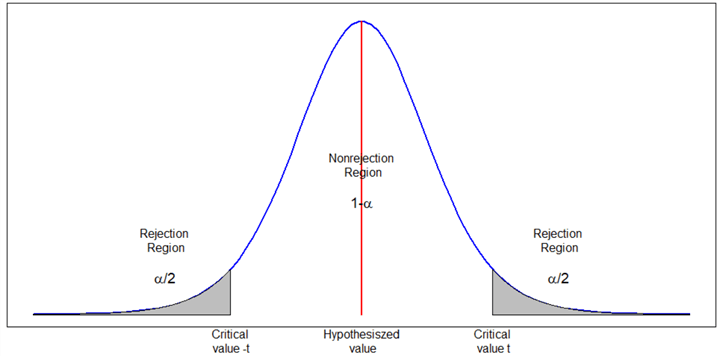
Figure 3 Critical regions for two-tailed tests
The second null hypothesis mentioned in Section 1.1 is that the average annual income for Adventure Works Cycles prospective customers is less than or equal to $50,000:
We test the null hypothesis ![]() against the alternate hypothesis
against the alternate hypothesis ![]() . Our concern is that the true mean may be higher than 50,000. Samples with a test statistic in the right tail area, shown in Figure 4, are used to reject the null hypothesis. This test is called a right-tailed test, which is appropriate for an alternative hypothesis involving a “greater than” situation [9].
. Our concern is that the true mean may be higher than 50,000. Samples with a test statistic in the right tail area, shown in Figure 4, are used to reject the null hypothesis. This test is called a right-tailed test, which is appropriate for an alternative hypothesis involving a “greater than” situation [9].
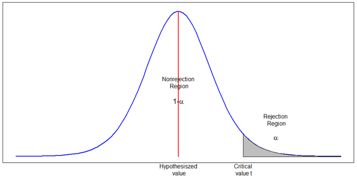
Figure 4 Critical regions for right-tailed tests
When samples with test statistics in the left tail (shown in Figure 5), are used to reject the null hypothesis, the test is called a left-tailed test. A left-tailed test is appropriate for an alternative hypothesis involving a “less than” situation [9].
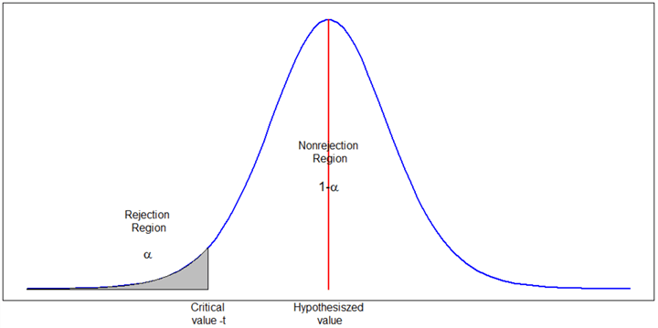
Figure 5 Critical regions for left-tailed tests
Since equality is usually part of the null hypothesis, we use the alternative hypothesis to determine whether we perform a right-tailed test or a left-tailed test. In practice, we may have this hypothesis:
Since the alternative hypothesis involves the “greater than” situation, a right-tailed test is required. The alternative hypothesis reflects a more specific concern. Samples with a sample mean less than 50,000 are not of interest, and we don’t use them as evidence to reject the null hypothesis in favor of the alternative hypothesis.
1.5 P-Value
To explain the concept of the p-value, let’s assume that the null hypothesis is true, the test statistic of an obtained sample is t, and we adopt one sampling process. The p-value of the statistical test is the probability of obtaining a sample with a test statistic value as extreme as or more extreme than the value of t [11]. Figure 6 shows the p-value of the right-tailed test, which is the area under the curve over the interval ![]()
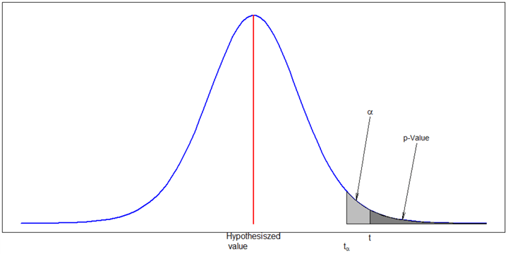
Figure 6 A right-tailed test using a p-value
We have defined the null hypothesis that the cameras installed in traffic intersections did not affect vehicle collisions. To test the null hypothesis, we select a sample denoted by X. Assuming the test result returns a p-value of .05, we interpret the p-value in terms of a hypothetical repetition of the experiment. We use the same sampling process to obtain more samples. If the null hypothesis is true, the p-value of .05 means 95% of samples demonstrate an effect smaller than sample X, and 5% of samples show the impact as the same as or larger than the sample X.
The p-value is defined formally as the probability of observing a value of the test statistic at least as contradictory to the null hypothesis as the observed test statistic value, assuming the null hypothesis is true [12]. The farther the test statistic is on the tails of the sampling distribution, the smaller the p-value is, and the stronger evidence to reject the null hypothesis. With a predetermined significance level α, we reject the null hypothesis if the p-value is less than α, and we do not reject the null hypothesis otherwise. It is worth noting that the misinterpretation of a p-value sometimes happens. [4] provides a guide to interpret the p-value correctly.
A p-value expresses the level of statistical significance: the smaller the p-value, the stronger the evidence against the null hypothesis if the underlying assumptions used to calculate the p-value hold. Dr. Hooper uses descriptive language to report the strength of the evidence [13]. Table 3 demonstrates the p-value interpretation provided by Dr. Hooper.
| p-value | Interpretation |
|---|---|
| >0.10 | No evidence against the null hypothesis. The data appear to be consistent with the null hypothesis. |
| (0.05, 0.10] | Weak evidence against the null hypothesis in favor of the alternative. |
| (0.00, 0.05] | Moderate evidence against the null hypothesis in favor of the alternative. |
| (0.001, 0.01] | Strong evidence against the null hypothesis in favor of the alternative. |
| <=0.001 | Very strong evidence against the null hypothesis in favor of the alternative. |
Table 3 P-value interpretation
1.6 Statistical Conclusion
Statistical hypothesis testing is a process of using a random sample to describe and make inferences about the population from which we produce the sample. We define a null hypothesis that reflects the status quo and an alternative hypothesis that shows our concerns. We want to assess the degree of evidence that the sample provides against the null hypothesis and, then, determine whether we have enough evidence to reject it [14].
An example of the status quo is that the coin in my hand is fair. My concern is that the coin is not fair. I flip the coin 100 times and get 55 heads. Because of randomness, this experiment result is reasonable if the coin is fair. However, I cannot say the null hypothesis is true because an unfair coin with probability 0.55 of landing heads up also can produce this result. If I get 90 heads from the experiment, I would doubt the null hypothesis because a fair coin is extremely unlikely to land heads up 90 times in this experiment. I cannot guarantee the alternative hypothesis is true either because a fair coin does have a chance to land heads up 90 times in 100 trials. Nevertheless, this experimental result demonstrates that the alternative hypothesis is much more plausible than the null hypothesis. Therefore, I can reject the null hypothesis intuitively.
When I get 55 heads, the experiment result appears to be consistent with the null hypothesis if the null hypothesis is true. However, when I get 90 heads, the null hypothesis seems not plausible if the underlying assumption holds. A threshold somewhere from the range 55-90 makes us start to doubt the null hypothesis and, consequently, rejects the null hypothesis. To determine the threshold, we calculate the value of the test statistic. Based on several factors, including the test statistic, the rejection region, the p-value, and the significance level, we can decide to reject the null hypothesis. When the test statistic is in the rejection region, or the p-value is less than or equal to the significance level, we reject the null hypothesis. Otherwise, we say we fail to reject the null hypothesis.
Statistical significance does not indicate a scientifically or substantively significant relation has been detected [4]. The statistical test does not demonstrate the degree of effect in the area of study. Subject-matter experts need to apply their knowledge and expertise to determine whether the test result is meaningful in practice.
2 – Statistical Hypothesis Testing of a Mean
Marketing managers in Adventure Works Cycles [1] are concerned that the average annual income of prospective customers increases to more than $50,000. To confirm this concern, the company needs to know the yearly dollar amount of income from all potential customers and, then, compute the average. This task is almost impossible. This demand motivates the need for a hypothesis test about a population mean. To prepare for the hypothesis test, we select a sample from the population. Then, we follow the 5-step process to perform the hypothesis test. The null hypothesis, stated in Section 1.1, is that the average annual income for Adventure Works Cycles prospective customers of is less than or equal to $50,000:
The alternative hypothesis — ![]() — involves a “greater than” situation, and therefore the test is right-tailed. More specifically, marketing managers want to use the sample data to perform a right-tailed test at a significance level of 0.05. The following R script is to choose 35 sampling units and, then, compute the sample mean and the sample standard deviation:
— involves a “greater than” situation, and therefore the test is right-tailed. More specifically, marketing managers want to use the sample data to perform a right-tailed test at a significance level of 0.05. The following R script is to choose 35 sampling units and, then, compute the sample mean and the sample standard deviation:
# Reset the compute context
to your local workstation.
rxSetComputeContext("local")
# Define the connection
string to SQL Server
sql.server.conn.string <-
"Driver=SQL Server;Server=.;Database=AdventureWorksDW2017;Trusted_Connection={Yes}"
# Create a RxSqlServerData
data source object
data.source.object <- RxSqlServerData(sqlQuery
= "
SELECT YearlyIncome
FROM [dbo].[ProspectiveBuyer]
",
connectionString = sql.server.conn.string)
# Read the data into a data
frame in the local R session.
data.frame.yearly.income <- rxImport(data.source.object)
# Set the seed of R random
number generator
set.seed(314159)
# Draw 35 sampling units
randomly from the population
sample.income <- sample(data.frame.yearly.income$YearlyIncome,
size = 35, replace =
FALSE)
# Compute mean and standard
deviation of the sample
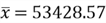
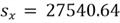
sample.mean <- mean(sample.income)
sample.standard.deviation <- sd(sample.income)
print(paste("sample
mean is: ", sample.mean))
print(paste("sample
standard deviation is: ", sample.standard.deviation))
The output in the R interactive window shows the results:
+
Rows Read: 2059, Total Rows Processed: 2059, Total Chunk Time: 0.083 seconds
[1] "sample mean is:  53428.5714285714"
[1] "sample standard deviation is:  27540.6498644818"
>
Since the sample size is greater than 30, the sampling distribution of means is approximately normal, and therefore the associated hypothesis test is called a z-test. Here is a list of inputs for the z-test:
- Sample size:

- Sample mean:
- Sample standard deviation:
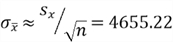
- Standard error of mean:
- Null hypothesis value:

- The level of significance:

We follow the 5-step process to perform the right-tailed test:
Step 1: State the null and alternative hypotheses:
Step 2: Compute the test statistic:
Step 3: Compute the (1-α) confidence interval for the test statistic z:
This hypothesis test is right-tailed, and therefore the 95% confidence interval is one-sided. The standard normal distribution table tells us that the critical value is 1.64 when α = 0.05. Here is the 95% upper one-sided confidence interval for the test statistic:
Testing the hypothesis is equivalent to checking whether the test statistic is in the confidence interval [5]. The test rejects the null hypothesis if, and only if, the test statistic is not in the confidence interval.
Step 4: State the technical conclusion:
Since the value of the test statistic, 0.74, is in the interval ![]() , the test statistic is in the nonrejection area. The sample data do not provide enough evidence to reject the null hypothesis; we fail to reject it at a significance level of 0.05. Thus, there is no significant evidence that the average annual income of prospective customers increases to more than $50,000.
, the test statistic is in the nonrejection area. The sample data do not provide enough evidence to reject the null hypothesis; we fail to reject it at a significance level of 0.05. Thus, there is no significant evidence that the average annual income of prospective customers increases to more than $50,000.
Step 5: Compute p-value:
When we repeat this experiment by using the same sampling process to obtain more samples, if the true population mean is 50,000, the chance of having a sample mean no less than 53428.57 is 23%. According to Table 3, there is no evidence against the null hypothesis; the sample data appear to be consistent with the null hypothesis. Besides, the p-value is higher than α. Therefore, we fail to reject the null hypothesis at a significance level of 0.05.
The manual process helps to enhance our understanding of statistical hypothesis testing. In practice, we often use the function “t.test” provided by R language to perform the test. Append the following two lines to the previous R code, then run the script:
# Perform one-sample t-test.
ttest <- t.test(x = sample.income, y
= NULL,
alternative ="greater",
mu = 50000, paired =
FALSE, conf.level = 0.95)
print(ttest)
The output in the R interactive window agrees with the results from the manual
calculation process. That is, the sample does not provide enough evidence to
reject the null hypothesis.
One Sample t-test
data:
sample.income
t = 0.7365, df = 34, p-value = 0.2332
alternative hypothesis: true mean is greater
than 50000
95 percent confidence interval:
45556.95
Inf
sample estimates:
mean of x
53428.57
3 – Statistical Hypothesis Testing of a Proportion
Historical data reveal that 60% of all Adventure Works Cycles [1] customers own a house. Before marketing managers promote a marketing strategy, they want to determine whether there is a change in the proportion. The null hypothesis reflects the logical opposite of their concern; the null hypothesis, defined in Section 1.1, is that the proportion of house owners is equal to 60%:
The alternative hypothesis — ![]() — involves a “not equal to” situation, and therefore the test is two-tailed. Marketing managers want to pick a sample from the population to perform a two-tailed test at a significance level of 0.05. The following R script is to take 35 sampling units and then compute the proportion of house owners in the sample:
— involves a “not equal to” situation, and therefore the test is two-tailed. Marketing managers want to pick a sample from the population to perform a two-tailed test at a significance level of 0.05. The following R script is to take 35 sampling units and then compute the proportion of house owners in the sample:
# Reset the compute context
to your local workstation.
rxSetComputeContext("local")
# Define connection string
to SQL Server
sql.server.conn.string <-
"Driver=SQL Server;Server=.;Database=AdventureWorksDW2017;Trusted_Connection={Yes}"
# Create an RxSqlServerData
data source object
data.source.object <- RxSqlServerData(sqlQuery
= "SELECT
CAST([HouseOwnerFlag] AS int) as
HouseOwnerFlag FROM [dbo].[ProspectiveBuyer]",
connectionString = sql.server.conn.string)
# Read the data into a data
frame in the local R session.
data.frame.HouseOwnerFlag <- rxImport(data.source.object)
# Set the seed of R random
number generator
set.seed(314)
# Draw 35 sampling units
randomly from the population
sample.size <-35
sample.HouseOwnerFlag <- sample(data.frame.HouseOwnerFlag$HouseOwnerFlag,
size = sample.size, replace =
FALSE)
# Compute the proportion
of house owners in the sample
success.number <- sum(sample.HouseOwnerFlag)
proportion <- success.number / sample.size
print(paste("the
proportion of house owners in the sample: ",
proportion))
The output in the R interactive window shows that the sample proportion is 51.4%:
Rows Read: 2059, Total Rows Processed: 2059,
Total Chunk Time: 0.003 seconds
[1] "the proportion of house owners
in the sample:
0.514285714285714"
When ![]() and
and ![]() , we can use a normal distribution to approximate the binomial distribution [9]. Since we have known,
, we can use a normal distribution to approximate the binomial distribution [9]. Since we have known, ![]() and
and ![]() , the test is a z-test. Besides, there are 18 successes in the sample of size 35; the test does not need to consider the continuity correction factor. Here is a list of inputs for the test:
, the test is a z-test. Besides, there are 18 successes in the sample of size 35; the test does not need to consider the continuity correction factor. Here is a list of inputs for the test:
- Sample size:
- Sample proportion:

- Null hypothesis value:

- The level of significance:
We follow the 5-step process to perform the two-tailed test:
Step 1: State the null and alternative hypotheses:
Step 2: Compute the test statistic:
Step 3: Compute (1-α) confidence interval for the test statistic z:
This a two-tailed test, and therefore the 95% confidence interval is two-sided. The standard normal distribution table indicates that the critical value is 1.96 when α = 0.05. Thus, the 95% confidence interval for the test statistic is [-1.96, 1.96].
Step 4: State the technical conclusion:
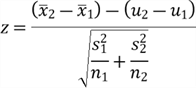
Since the test statistic -1.04 lies in the interval [-1.96, 1.96], the test statistic is in the nonrejection area. The sample data do not provide enough evidence to reject the null hypothesis; therefore, we fail to reject the null hypothesis at a significance level of 0.05. Consequently, we have no significant evidence that there is a change in the proportion of house owners.
Step 5: Compute p-value:
Use the standard normal distribution table to find the probability in the left tail:
By the symmetry of the normal curve, we look at the probability in the right tail:
Therefore
If the true population proportion is 0.6, there is a 30% chance of observing a sample with a proportion of house owners no more than 0.514 or no less than 0.686. Since the probability of selecting such a sample is not extremely low, we do not think that the sample data provide compelling evidence to reject the null hypothesis. According to Table 3, there is no evidence against the null hypothesis; the sample data appear to be consistent with the null hypothesis when the null hypothesis is true. Besides, the p-value is higher than α. Therefore, we fail to reject the null hypothesis at a significance level of 0.05.
We use the R functions prop.test() to perform the one-proportion test when the sample size is more than 30. I append the following two lines to the previous R script, then run the script. I explicitly set the argument “correct” to False because this test does not consider the continuity correction factor.
# Perform one proportion
z-test.
ptest <- prop.test(x = success.number,
n = sample.size, alternative =
"two.sided",
p = 0.6, conf.level = 0.95, correct =
FALSE)
print(ptest)
The output in the R interactive window agrees with the results from the manual
calculation process. That is, the sample does not provide enough evidence to
reject the null hypothesis.
1-sample proportions
test without continuity correction
data:
success.number out of sample.size,
null probability 0.6
X-squared = 1.0714, df = 1, p-value = 0.3006
alternative hypothesis: true p is not equal
to 0.6
95 percent confidence interval:
0.3556880
0.6700576
sample estimates:
p
0.5142857
>
4 – Commonly Used Hypothesis Tests
We have performed two hypothesis tests and illustrated the process of hypothesis testing. There are other types of hypothesis tests. Rumsey [14] has summarized the most common hypothesis tests. In her book, she provided formulas, explained the calculations, and walked through some examples.
Professor Jost has compiled six commonly used hypothesis tests [2]:
- One-sample z-test
- One-sample t-test
- Paired-sample z-test
- Paired-sample t-test
- Independent Two-sample z-test
- Independent Two-sample t-test
When the sample size is large (n > 30), the central limit theorem (CLT) states that the distribution of the sample means is approximately normal, even though all these independent observations from a population do not have a normal distribution. We use the formulas provided in Table 1 to compute a test statistic and perform a z-test.
When a sample has a small size (n ≤30), CLT does not apply to it. We can perform a t-test when the original population is approximately normal. The test statistic, computed by formulas in Table 1, has a t-distribution with (n-1) degrees of freedom.
Even though we can use the 5-step process to perform these six commonly used hypothesis tests, the computation of test statistic varies from test to test. Naghshpour [15] provided a table to present test statistic computations for testing hypotheses. For example, an independent two-sample z-test uses the following formula to compute the test statistic:
Many statistics books introduce these formulas, and some modern tools provide functions to perform these tests. This tip aims to introduce fundamental concepts behind statistical hypothesis testing; then, we can build useful models and give plausible statistical conclusions. Larry mentioned that using fancy tools without understanding basic statistics is like doing brain surgery before knowing how to use a band-aid [5].
Summary
Statistical hypothesis testing allows us to determine whether to reject some assumptions about a population according to information from a sample. We started the tip with a problem statement. We want to help marketing managers to determine whether a sample selected from the population provides enough evidence to reject status quos. The solution is to follow a 5-step process to test these hypotheses.
The elements involved in this 5-step process are null hypothesis, alternative hypothesis, test statistic, level of significance, rejection region, p-value, and statistical conclusion. After an overview of these elements, we conducted a right-tailed test at a significance level of 0.05 on whether there is sufficient evidence that the average annual income for Adventure Works Cycles prospective customers has increased. We walked through the 5-step process step by step; then, we demonstrated how to perform the test by using the “t.test()” function in R.
Next, we constructed a two-tailed hypothesis test of a proportion at a significance level of 0.05 on whether there is sufficient evidence that the percentage of house owners in all prospective customers has changed. The sample size and sample proportion met conditions for using the normal distribution to approximate the binomial distribution. We applied the 5-step process again. Then, the function “prop.test()” in R helps to confirm the manual calculation process.
Finally, we glanced at some commonly used hypothesis tests. We can continue to use this 5-step process, but the test statistic computation varies from test to test.
References
[1] Kess, B. (2017). AdventureWorks sample databases. Retrieved from GitHub: https://github.com/Microsoft/sql-server-samples/releases/tag/adventureworks/.
[2] Jost, S. (2017). CSC 423: Data Analysis and Regression. Retrieved from DePaul University: http://facweb.cs.depaul.edu/sjost/csc423/
[3] Freund, J. R., Mohr, D. & Wilson, J. W. (2010). Statistical Methods. Burlington, MA: Academic Press
[4] Greenland, S., Senn, J. S., Rothman, J. K., Carlin, B. J., Poole, C., Goodman, N. S. & Altman, G. D. (2016). Statistical Tests, P values, Confidence Intervals, and Power: A Guide to Misinterpretations. Eur J Epidemiol, 31: 337-450.
[5] Wasserman, L. (2004). All of Statistics: A Concise Course in Statistical Inference. New York, NY: Springer
[6] Doren, V. C. (1991). A History of Knowledge: Past, Present, and Future. New York, NY: Random House
[7] Helmenstine, M. A. (2020). Six Steps of the Scientific Method. Retrieved from ThoughtCo: https://www.thoughtco.com/steps-of-the-scientific-method-p2-606045.
[8] Garber, J. N., Miller, S. J., Abel, E. R., Eslambolchi S. & Korukonda, K. S. (2007). Final Report: The Impact of Red Light Cameras (Photo-Red Enforcement) on Crashes in Virginia. Retrieved from virginiadot.org: http://www.virginiadot.org/vtrc/main/online_reports/pdf/07-r2.pdf.
[9] Hummelbrunner, S. A., Rak, L. J., Fortura, P., & Taylor, P. (2003). Contemporary Business Statistics with Canadian Applications (3rd Edition). Toronto, ON: Prentice Hall.
[10] Smith, Y. (2019). Type I and Type II errors of hypothesis tests: understand with graphs. Retrieved from Towards Data Science: https://towardsdatascience.com/type-i-and-type-ii-errors-of-hypothesis-tests-understand-with-graphs-43079fdd936a/.
[11] Gibson, J. (2017). Calculate the P-Value in Statistics – Formula to Find the P-Value in Hypothesis Testing. Retrieved from Towards Data Science: https://youtu.be/KLnGOL_AUgA/.
[12] William, M., & Sincich, T. (2012). A Second Course in Statistics: Regression Analysis (7th Edition). Boston, MA: Prentice Hall.
[13] Hooper, P. What is a P-value? Retrieved from stat.ualberta.ca: http://www.stat.ualberta.ca/~hooper/teaching/misc/Pvalue.pdf.
[14] Rumsey, J. D (2011). Statistics for Dummies (2nd Edition). Indianapolis, IL: Wiley Publishing.
[15] Naghshpour, S. (2015). Statistics for Economics (2nd Edition). New York, NY: Business Expert Press
Next Steps
- Statistical hypothesis tests and p-values are still widely used, even though misinterpretation and abuse have been observed and discussed for many years. This tip has introduced basic concepts and test procedures. When we want to use them in practice, we should study them in more depth. I recommend the essay [4] that provide a guide to avoiding misinterpretations. For readers who want to gain in-depth knowledge about hypothesis testing, I strongly recommend the course “Statistics for Applications” taught at MIT by Professor Philippe Rigollet. Lecture videos are available within the course site.
- Check out these related tips:
- Basic Concepts of Probability Explained with Examples in SQL Server and R
- Using SQL Server RAND Function Deep Dive
- Selecting a Simple Random Sample from a SQL Server Database
- Numerically Describing Dispersion of a Data Set with SQL Server and R
- T-Test Add-on for the SQL Statistics Package
- Statistical Parameter Estimation Examples in SQL Server and R

Nai Biao Zhou has twenty years of experience in software development, with strong analytical skills and a broad range of computer expertise.
He has fifteen years of experience in development and maintenance of database applications on SQL Server in OLTP/OLAP/BI environments.
He has a master’s degree in Control Engineering and is pursuing a Master of Science degree in Predictive Analytics.
Knowledge/Skills
Advanced computer programming skills and well versed with C/C#, Java, ASP.NET, JavaScript, and SQL.
In depth knowledge of Solution Architecture, and Software Development Life Cycle (SDLC).
Microsoft Certified Application Developer (MCAD) since 2004.
- MSSQLTips Awards: Author of the Year – 2021 | Rising Star (50+ tips) – 2024 | Author Contender – 2020, 2023