Selecting a Simple Random Sample from a SQL Server Database

By: Nai Biao Zhou | Comments | Related: > TSQL

Problem

In the business world, useful information about a population usually is gathered by studying a selected portion of the population. The portion is called a sample, and the process of selecting the sample is called sampling. Sampling is a fundamental operation for auditing and statistical analysis of large databases [1]. Many people in the database community are required to select a sample from a SQL server database. A simple solution on the web is to use the SQL statement "ORDER BY NEWID()". This solution may not fit all populations. For example, in FM radio markets, a station considers the age group of the target audience as an important determinant for the type of programming [2]. If 30 listeners are chosen randomly from a SQL server database that contains all listeners through using this method, the sample may not include listeners of a certain age subgroup. Thus, the sample might misrepresent the population. Additional sampling techniques are required to reduce this sample selection bias. Those database professionals who are unfamiliar with statistics may want to know more sampling techniques and the nature of the uncertainties created by these sampling techniques.

Solution

To sensitize that sampling is not merely to select some random items from a population, I quoted a statement from William Edwards Deming [3]: Sampling is not a mere substitution of a partial coverage for total coverage. Sampling is the science and art of controlling and measuring the reliability of useful statistical information through the theory of probability. To explore this science and art, the tip is devoted to two topics: sampling techniques, and sampling distributions.

The focus of the first part is to introduce sampling techniques. Section 1.1 covers some basic concepts of sampling. Then, two categories of sampling techniques are briefly introduced in Section 1.2. Next, Section 1.3 adopts the lottery method of the simple random sampling to select a sample from a SQL server database.

The second part is devoted to sampling distributions. Section 2.1 explains the expected value and variance of a random variable. Sections 2.2 studies one of the most important theorems in statistics: The Central Limit Theorem (CLT). Section 2.3 introduces the well-known normal distributions. Section 2.4, then, studies variation among many samples. Finally, Section 2.5 briefly introduces the sample size determination technique.

All the source codes used in this tip were tested with SQL Server Management Studio V18.3.1, Microsoft Visual Studio Community 2017 and Microsoft R Client 3.4.3 on Windows 10 Home 10.0 <X64>. The DBMS is Microsoft SQL Server 2017 Enterprise Edition (64-bit).

1 – Sampling Techniques

When we study the characteristics of an entire population, because of physical constraints, economical constraints, time constraints or other constraints, it is usually impractical to gather information from every unit within a population. We use sampling techniques to estimate the characteristics of the entire population.

1.1 Basic Concepts of Sampling

To precisely explain sampling techniques, let’s study some definitions that were excerpted from [4,5,6].

Population: A population is a collection of data measured on all experimental units of interest to the researcher. The concept of experimental units herein refers to those objects upon which the measurements (or observations) are made. The collection of data, which is typically large, possibly infinite, either exists in fact or is part of an ongoing operation and hence is conceptual [4]. For example, the population could be "all customers of a manufacturer over the recent past and in the future".

Finite Population: A finite population is a population that consists of a finite number of experimental units.

Infinite Population: An infinite population is a population in which it is theoretically impossible to measure all the experimental units. In practice, a finite population with many experiment units is considered to be an infinite population.

Target Population: The complete collection of observations that the researcher wants to study [5]. The research objective determines the choice of the target population. For example, when we study customers of a manufacturer, the target population could be all individual customers, all corporate customers, or all registered customers. Each target population possesses its characteristics.

Sample: A sample is a subset of data selected from a population [4], which is representative of the population.

Sample Size: The number of experimental units to be included in a sample [6].

Sampling: The process of selecting a sample from the population is called sampling [6].

Sampling Unit: An experimental unit that is selected for a sample [5].

Sampled Population: The population from which the sample was taken [5]. Ideally, the sampled population is the same as the target population. In practice, the sampled population is usually smaller than the target population. For example, we want to study all customers of a retailer, i.e. target population. But not all customers have registered their personal information into the Customer Relationship Management (CRM) system. All those customers in the CRM system form the sample population.

Sampling Frame: A list, map, or other specification of sampling units in the population from which a sample may be selected [5]. The sampling frame differs from the population in that the sampling frame is more specific. For example, the sampling frame of the manufacturer customers is an actual list of all customers in the database tables. The population, on the other side, is abstract, for example, all customers of the manufacturer. We select a sample from the sampling frame rather than the population.

Parameters: Numerical descriptive measures of the population [4], for example, the population mean and the population standard deviation .

Statistics: Numerical descriptive measures calculated from sample data [4], for example, the sample mean and the sample standard deviation .

1.2 Sampling Techniques

Based on the method of selecting a sample, various sampling techniques are broadly categorized into two groups: probability sampling and non-probability sampling. When sampling techniques of probability sampling are used, sampling units are selected randomly by known probabilities from a sampling frame. On the other side, in non-probability sampling, each unit is selected without the use of probability. Some other factors, for example, the researcher’s judgment, convenience, etc. determine the selection of a sample.

Table 1 shows the broad classification of probability sampling and non-probability sampling. Most sampling solutions on the web provided by the database community are using the simple random sampling method. Database professionals can find an appropriate method in this table according to the nature of the population.

One purpose of this tip is to present a list of sampling techniques to database professionals. All these techniques bring risks of sampling errors. Depending on the nature of populations, some techniques might carry smaller risks of sampling errors. Furthermore, some techniques can predict the risks of sampling errors. A detailed exploration of each sampling technique is beyond the scope of this tip. In Section 1.3, we will give practice in the use of simple random sampling for selecting a sample.

1.3 Selecting a Simple Random Sample Without Replacement

A simple random sample (hereinafter referred to as the "SRS") is one of the simplest forms of probability sample, and it is the foundation for more complex sampling designs [5]. There are two ways of selecting a unit for a simple random sample: with replacement (hereinafter referred to as the "SRSWR") and without replacement (hereinafter referred to as the "SRSWOR"). In this tip, we will take a SRSWR. That means the units once chosen are not placed back in the sampling frame.

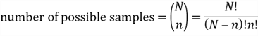
If we take samples of size from a population of size is , the total number of possible samples is computed by the combinations rule:

In a SRSWOR, every possible sample should have an equal chance of being selected as the representative of the population. Therefore, the probability of one sampling unit, such as unit , being selected into any samples is obtained by the following equation:

There are two methods of randomly selecting a sampling unit [6]:

The lottery method;
Using random numbers;

In the lottery method, each sampling unit is assigned a number. We select numbers one by one and all selected numbers will not be selected again. The process is analogous to drawing lottery numbers in a box. We can use a computer program to choose these sampling units randomly.

AdventureWorks is a fictional company that sells bicycles and cycling accessories. Microsoft provides a transactional database [8] with 27,659 online orders placed by individual customers. I have used the lottery method to take a SRSWOR of size 30 from this population.

The first step is to assign a number to each sampling unit. I created a temporary table with an identity column, then inserted all online orders placed by individual customers into the temporary table. This process assigned all orders with consecutive whole numbers:

CREATE TABLE #all_online_orders
(
  order_id      int identity(1,1) primary key,
  order_no      nvarchar(25) not null,
  customer_name nvarchar(150) not null,
  order_date    datetime not null,
  total_amount  money not null,
);
 
INSERT INTO #all_online_orders
SELECT so.[SalesOrderNumber]
         ,CONCAT(p.FirstName, ' '
         ,p.LastName) AS [Customer Name]
         ,so.[OrderDate]
         ,so.[SubTotal]
FROM [Sales].[SalesOrderHeader] so 
INNER JOIN [Sales].[Customer] sc ON so.CustomerID = sc.CustomerID
INNER JOIN [Person].[Person] p ON sc.PersonID = p.BusinessEntityID
WHERE so.[OnlineOrderFlag] = 1
  and so.[Status] = 5
  and sc.StoreID IS NULL
order by [OrderDate]

The second step is to generate random numbers. I used the 4-step procedure [9] for generating 30 random integer numbers from the range [1, 27659]. Note that duplicates were discarded. Comparing to the population size 27659, the sample size 30 is so small that the chance of generating numbers with duplicates is low.

CREATE TABLE #lottery_number 
( 
   lottery_number int primary key 
); 

WHILE (SELECT COUNT(*) FROM #lottery_number) < 30 
BEGIN 
   BEGIN TRY  
      INSERT INTO #lottery_number 
      SELECT CEILING(RAND(CHECKSUM(NEWID())) * 27659.0) 
   END TRY  
   BEGIN CATCH  
      PRINT 'discards duplicates' 
   END CATCH 
END

The last step is to select sampling units according to these random numbers. I used these random numbers to find their corresponding online orders, and therefore a SRSWOR has been selected:

SELECT 
    order_id, 
    order_no, 
    customer_name, 
    order_date, 
    total_amount 
FROM #all_online_orders o 
INNER JOIN #lottery_number l ON o.order_id = l.lottery_number

Table 2 shows the SRSWOR of size 30. It is noteworthy that we must resist a temptation of making any adjustment of the sample, even though some units in the sample does not look random.

Bajpai has provided a 5-step sampling design process in his book [6]: (1) define the target population; (2) determine the sampling frame; (3) select an appropriate sampling technique; (4) determine sample size; (5) execute the sampling process. Kabir also has summarized a 7-step sampling design process [10]. By following these systematic design processes, we have more chances to get a representative sample.

2 – Sampling Distribution

Table 2 showed the selected sample of size 30. I assume that the characteristic of interest is the total amount of each order. Using the sample mean and sample standard deviation definitions introduced in [11], the sample mean is 1,267.56 and the sample standard deviation is 1,244.96. When we repeatedly take a SRSWOR of size 30, we get different sample means and sample standard deviations. The following procedure was used to select 20,000 samples, calculate sample means, and then produce a histogram of the sample means:

Step 1: Run the following T-SQL script to compute sample means and save them into a global temporary table:

CREATE TABLE #all_online_orders 
( 
   order_id int identity(1,1) primary key, 
   order_no nvarchar(25) not null, 
   customer_name nvarchar(150) not null, 
   order_date datetime not null, 
   total_amount money not null, 
); 

CREATE TABLE #lottery_number 
( 
   lottery_number int primary key 
); 

CREATE TABLE  ##order_avg_amount  
( 
   avg_amount money not null 
); 

INSERT INTO #all_online_orders 
SELECT so.[SalesOrderNumber] 
      ,CONCAT(p.FirstName, ' ', p.LastName) AS [Customer Name] 
      ,so.[OrderDate] 
      ,so.[SubTotal] 
FROM [Sales].[SalesOrderHeader] so 
INNER JOIN [Sales].[Customer] sc ON so.CustomerID = sc.CustomerID 
INNER JOIN [Person].[Person] p ON sc.PersonID = p.BusinessEntityID 
WHERE so.[OnlineOrderFlag] = 1 and so.[Status] = 5 and sc.StoreID IS NULL 
order by [OrderDate] 

WHILE (select COUNT(*) from ##order_avg_amount) < 20000 
BEGIN 
   TRUNCATE TABLE #lottery_number 
   WHILE (select COUNT(*) from #lottery_number) < 30 
   BEGIN 
      BEGIN TRY  
         INSERT INTO #lottery_number 
         SELECT CEILING(RAND(CHECKSUM(NEWID())) * 27659.0) 
      END TRY  
      BEGIN CATCH  
         print 'disregards duplicates' 
      END CATCH 
   END 
   INSERT INTO ##order_avg_amount 
   SELECT AVG(total_amount) as avg_amount 
   FROM #all_online_orders o 
   INNER JOIN #lottery_number l ON o.order_id = l.lottery_number 
END 
DROP TABLE #lottery_number 
DROP TABLE #all_online_orders

Step 2: Run the following R script to retrieve data from the global temporary table and then plot a histogram:

# Reset the compute context to your local workstation. 
rxSetComputeContext("local") 
# Define connection string to SQL Server 
sql.server.conn.string <- "Driver=SQL Server;Server=.;Database=AdventureWorks2017;Trusted_Connection={Yes}" 
# Create an RxSqlServerData data source object 
data.source.object <- RxSqlServerData(sqlQuery = "                                     
                                select avg_amount from ##order_avg_amount 
                                ", 
                                connectionString = sql.server.conn.string) 
# Read the data into a data frame in the local R session. 
data.frame.avg.amount <- rxImport(data.source.object) 
# Create a Histogram of Random Numbers 
hist(data.frame.avg.amount$avg_amount, main = "The Histogram of Sample Means", 
     xlab = "Sample Mean", freq = TRUE)

Step 3: Drop the global temporary table:

DROP TABLE ##order_avg_amount

Figure 1 The Histogram of Sample Means

Figure 1 exhibits the frequency distribution of sample means. The histogram is close to a bell-shaped curve. To have a better understanding of the variability in these sample statistics, and then to estimate population parameters, we need to study the probability distributions of these statistics, called sampling distributions. In this tip, I place my focus on the sampling distribution of the means.

2.1 Expected Value and Variance

I have explored discrete probability distributions and continuous probability distributions in [9]. Through probability distributions, we can compute the chance of a random variable taking a value within a range. This section studies some measures of the probability distributions: expected value, variance and standard deviation.

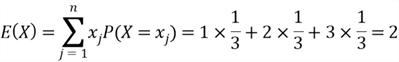
When we arrange a set of observations into an array, one measure of the array is the mean of the array. The mean is a central value around which the data tend to cluster. The probability distribution of a continuous random variable also has some descriptive measures such as expected value. The expected value is the mean of a random variable that represents the mean outcome when we repeat a random experiment many times. The expected value of a discrete random variable is defined by:

where is the random variable with distinct possible values ; is the size of the support, possibly infinitely; is the probability mass function(PMF).

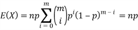
The discrete uniform distribution, the Bernoulli distribution, and the binomial distribution have been discussed in [9]. We use PMFs of these distributions to compute expected values of these random variables:

(1), has a discrete uniform distribution, denoted by .

(2), has a Bernoulli distribution, denoted by .

(3), has a binomial distribution, denoted by .

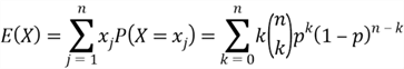
Let and , then

The probability distribution of a continuous random variable does not have a PMF, instead, it has a probability density function (PDF). We interpret the expected value of a continuous random variable in the same way as we did for the discrete random variables. The expected value is the mean value of the continuous random variable over a large number of experiments. The expected value of the continuous random variable is computed by

where is the random variable with PDF .

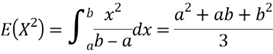
The PDFs of uniform distribution and the standard distribution have been given in [9]. We use these PDFs to calculate expected values of these random variables:

(1), has a uniform distribution, denoted by .

(2), has the standard normal distribution, denoted by .

Before computing the expected value, let’s review some properties of a function . If is an odd function and the integral of the odd function exists, the area under the function from -a to 0 cancels the area under the function from 0 to a:

If is an even function, and the integral of the even function exists, the area under the function from -a to 0 is equal to the area under the function from 0 to a:

Since is an odd function, therefore the expected value of the standard normal random variable is 0:

The most important property of expected value is linearity, which is represented by the following equations [7]:

Variance and standard deviation, the most widely used measures of variability, describe the dispersion of a random variable. The variance is the average of the squared deviations about the expected value of the random variable, and the standard deviation is the positive square root of the variance:

The variance of random variables has some useful properties. If and are independent continuous random variables, the variance of the random variable is obtained by the following equation [7]:

If is a continuous random variable and is a constant, the variance of the random variable is obtained by the following equation [7]:

Since we have already calculated expected values of some random variables, we use these expected values to compute variances of random variables:

(1), has a discrete uniform distribution, denoted by .

(2), has a Bernoulli distribution, denoted by .

(3), has a binomial distribution, denoted by .

The process to compute the is not straightforward. We have already known that a binomial distribution with parameters and can be considered to perform independent Bernoulli trials with the probability of success in each trial. We use to denote a success of the trial, then can be represented by:

It is noting that all random variables from have the same value of variance, that is . Then, we can use the property of variance to compute the variance of the random variable :

(4), has a uniform distribution, denoted by .

(5), has the standard normal distribution, denoted by .

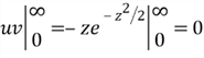
Assuming that we have already known the following two equations, we use them to compute the variance of the standard normal distribution. The proof of the first equation is very tricky and requires more mathematical background. The second equation uses the fact that decays much faster than grows [7].

Then, we compute the term in the variance equation:

Let and , then

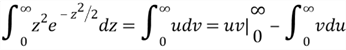
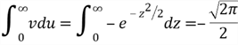
Therefore,

2.2 The Central Limit Theorem

Let’s represent the characteristic of each unit in a population by a random variable , and assume are independent, identically distributed with finite mean and finite variance . The mean of the sample of size is computed by

The sample mean is a random variable because a function of random variables is a random variable. When we repeatedly take a sample of size from the population, we obtain different sample means and sample standard deviations. We compute expected value and variance of the sample means:

We usually denote the expected value of the sample means by and denote the standard deviation of the sample means by , which is also referred to as the standard error of the mean. We denote the standard error of the mean by . Then, we have these equations:

The law of large numbers (LLN) says that, as the sample size , the sample mean converges to the true mean pointwise with probability 100% [7]. LLN has two versions, and the proof of the weak law of large numbers is provided in book [7]. We have implicitly applied LLN in many simulations already. For example, I repeatedly ran programming scripts in [9] to find the probability of event occurrences.

The central limit theorem (CLT) describes the distribution of the random variable :

Random variables are independent and identically distributed with mean and variance . If these random variables constitute a random sample from an infinite population, as , the distribution of approaches standard normal.

To prove this theorem, we need to have some knowledge of the moment generating function (MGF), which is not required in this tip. In practice, we often use the approximation form of the CLT: for a large , the distribution of is approximately normal distributed, denoted as . Usually, we consider sample size to be large if . The approximation form of the CLT states that even if independent observations from a population that is not normally distributed, the sample mean of the observations is approximately normally distributed if is large.

2.3 Normal Distributions

The three main reasons make normal distributions be a keystone in statistics [12]:

Many random variables in science, business and industry are approximately normally distributed;
The shape of some discrete probability distributions approximates a normal distribution when the size of the support is large enough;
The central limit theorem provides the basis for statistical inference;

Normal Distributions have the well-known bell-shaped curve shown in Figure 2. They have the probability density function (PDF) with two parameters and :

When a random variable has this PDF, the variable has a normal distribution and it is referred to as a normal random variable.

Figure 2 Normal Probability Density Function

The following are some of the important characteristics of the normal curve [12,13]:

The curve is bell-shaped and has one peak at the center of the distribution, on which the mean, median and mode locate;
The curve is symmetrical about the mean . The area under the curve to the left of the mean equals to the right of the mean;
The curve has inflection points at and , where is the standard deviation;
The area under the curve represents probability. The total area under the curve is 1. The area lies within the interval from to is about 68%. The area lies within the interval from to is about 95%. The area lies within the interval from to is about 99.7%.

Since both PDF and CDF of normal distributions are not closed-form expressions, it is not effective to compute the area under the curve by using these two functions. In practice, we transform a normal distribution into the standard normal distribution, denoted by , which has a mean of 0 and a variance of 1:

where is called z-score or z-value that represents the distance from the mean in standard deviation units, and is the value of the random variable .

The areas under the standardized normal curve have been tabulated. We also can compute the areas by using a built-in function in programming languages, for example, R language. Let’s look at an example in [13]:

Let be , where the random variable represents the length of life (in years) of an electric can opener. If this can opener has a 1 yr warranty, what fraction of original purchases will require replacement? (Panik, 2012, Example 6.3)

I would like to point out that in book [13] denotes that normal distribution has a mean of 2.9 and a standard deviation of 0.9. Other books, for example [7], interprets that the normal distribution has a variance of 0.9. In this example, I consider that the distribution has a standard deviation of 0.9 so that the answer is the same as the one in book [13].

First, we transform the normal distribution into the standard normal distribution :

The question asked to find the probability when . Let’s express in terms of :

The gray area in Figure 3 represents the probability. We can either use the table of probabilities and Z-scores or use a computer program to compute the gray area. I used the following R function, and the function returned a value of 0.0174. It seems about 1.74% of original sales will require replacement because of the 1-year warranty.

> pnorm(-2.11, lower.tail = TRUE) 
[1] 0.01742918

Figure 3 The Area to the Left of (z=-2.21)

2.4 Sampling Distribution of the Means

Figure 1 plotted means of 20,000 samples and illustrated the sampling distribution of the means. We usually cannot produce all possible sample means to study the sample distributions of the means. Statistical theory concludes three important characteristics of the sampling distribution of the means [14]:

Because of the CLT, if the sample size is large (rule of thumb ), the sample means are approximately normally distributed, even though the population does not have a normal distribution;
The mean of the sampling distribution of the means is equal to the population mean:

The standard deviation of the sampling distribution of the means, commonly referred to as the standard error, is computed as the population standard deviation divided by the square root of the sample size when the population is infinite:

The finite correction factor is used for a finite population:

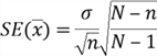
In practice, the finite correction factor usually is ignored unless [12].

Because the population standard deviation usually is unknow, is estimated by the sample standard deviation if the sample size is greater than 30 [14,15]:

We have defined a population with 27,659 online orders placed by individual customers. I used the following T-SQL statement to find the populations parameters:

SELECT AVG([SubTotal])  AS Mean 
   ,VAR([SubTotal]) AS Variance 
   ,COUNT(*) AS N 
FROM [Sales].[SalesOrderHeader] so JOIN [Sales].[Customer] sc ON so.CustomerID = sc.CustomerID 
WHERE so.[OnlineOrderFlag] = 1 
and so.[Status] = 5 
and sc.StoreID IS NULL

The population has a mean of 1061.45, a variance of 1320260.75 and a standard deviation of 1149.03. When we select an SRSWOR of size 30 from the population, Let’s find the probability that the difference between the sample mean and the population mean is not over 5% of the population mean:

We have already known

Compute the range of the z-scores

The probability of the event as shown in Figure 4 was computed by the following R commands:

> 1-2*pnorm(-0.26, lower.tail = TRUE) 
[1] 0.2051362 
>

Figure 4 The Probability of the Event P(-0.26≤z≤0.26)

There are 20.5% of the chance that the sample mean is in the interval , i.e. [1008.377, 1114.523]. To verify the theorical calculation, I use T-SQL script to select 20,000 samples, then compute the probability of the sample mean being in this interval. The following script returned the probability of 20.7%, which is close to the theoretical calculation.

CREATE TABLE #all_online_orders 
( 
   order_id int identity(1,1) primary key, 
   order_no nvarchar(25) not null, 
   customer_name nvarchar(150) not null, 
   order_date datetime not null, 
   total_amount money not null, 
);
 
CREATE TABLE #lottery_number 
( 
   lottery_number int primary key 
);
 
CREATE TABLE  ##order_avg_amount  
( 
   avg_amount money not null, 
   within_interval smallint not null 
); 

INSERT INTO #all_online_orders 
SELECT so.[SalesOrderNumber] 
      ,CONCAT(p.FirstName, ' ', p.LastName) AS [Customer Name] 
      ,so.[OrderDate] 
      ,so.[SubTotal] 
FROM [Sales].[SalesOrderHeader] so INNER JOIN [Sales].[Customer] sc ON so.CustomerID = sc.CustomerID 
INNER JOIN [Person].[Person] p ON sc.PersonID = p.BusinessEntityID 
WHERE so.[OnlineOrderFlag] = 1 and so.[Status] = 5 and sc.StoreID IS NULL 
order by [OrderDate] 

WHILE (select COUNT(*) from ##order_avg_amount) < 20000 
BEGIN 
   TRUNCATE TABLE #lottery_number 
   WHILE (select COUNT(*) from #lottery_number) < 30 
   BEGIN 
      BEGIN TRY  
         INSERT INTO #lottery_number 
         SELECT CEILING(RAND(CHECKSUM(NEWID())) * 27659.0) 
      END TRY  
      BEGIN CATCH  
         print 'disregards duplicates' 
      END CATCH 
   END 
   INSERT INTO ##order_avg_amount 
   SELECT AVG(total_amount) as avg_amount, 
      IIF(AVG(total_amount) >= 1008.377 and AVG(total_amount) <= 1114.523, 1, 0) 
   FROM #all_online_orders o 
   INNER JOIN #lottery_number l ON o.order_id = l.lottery_number 
END 

SELECT CAST(SUM(within_interval) as float)/CAST(COUNT(*) as float) AS probability 
FROM ##order_avg_amount 

DROP TABLE #lottery_number 
DROP TABLE #all_online_orders 
DROP TABLE ##order_avg_amount

2.5 Determining Sample Size

The sample size is the number of units selected for a sample. Based on the definition of the standard error of the sample mean, as the sample size increases, the standard error decreases. However, a larger sample size means more cost of sampling. Determination of sample size is one of the most important steps in the sampling process. To determine the sample size, we should at least know these two criteria:

The level of precision, which is a range to include the true value of the population. For example, we may need to determine a sample size so that the estimate mean should be within 5% error of the true mean;
The confidence level, which describes the uncertainty associated with a sampling method. We cannot guarantee a single sample to be representative of the population. The true mean may not in the estimated interval by using the single sample. A confidence level, for example, 95%, means that, by repeating the procedure over and over again, we obtain many computed intervals, and 95% of these intervals contain the true mean.

When determining the size of the sample, a typical requirement is that the estimate should be within a 5% error of the true parameter. [16, 17] review other criteria: the purpose of the study, the population size, the degree of variability in the attributes being measured [18], the statistical power and one- or two-tailed statistical analysis.

[16,17] also have covered several approaches to determine the sample size: using a census for small populations, imitating a sample size of similar studies, using published tables, and applying formulas to calculate the sample size.

Summary

A population is a collection of data measured on all experimental units of interest to the researcher. A sample is a subset of data selected from a population. The researcher usually studies samples to gather useful information about the population. The two main types of sampling techniques are probability sampling and non-probability sampling. In the probability sampling process, the probability of units being selected into the sample is known. In non-probability sampling methods, the chance of units being selected within the population is unknown. A typical sampling technique is the simple random sampling without replacement.

The expected value represents the mean outcome when we repeat a random experiment many times. In the inferential process, sample means are used to estimate population means because of the central limit theorem. The central limit theorem states that for a population with any distribution shape if a sample of sufficiently large sample size n (n ≥30) is drawn from the population, the sample means are approximately normally distributed.

The probability density function (PDF) of a normal distribution is the well-known bell-shaped curve, which is symmetrical about its mean and asymptotic to the horizontal axis. The two parameters mean and standard deviation together determine a normal probability distribution. The mean of the sampling distribution of the means is equal to the population mean, and the standard deviation of the sampling distribution of the means is computed as the population standard deviation divided by the square root of the sample size.

Sample size determination is the technique of determining the number of units selected for a sample. The level of precision and the confidence level need to be specified to determine the appropriate sample size. Several strategies are available to determine sample size, such as using a census for small populations, imitating a sample size of similar studies, using published tables, and applying formulas to calculate the sample size.

References

[1] Olken, F., & Rotem, D. (1986). Simple Random Sampling from Relational Databases. VLDB.

[2] Black, K. (2013). Business Statistics: For Contemporary Decision Making, 8th Edition. Hoboken, NJ: Wiley.

[3] Deming, W. E. (1950). Some Theory of Sampling. Mineola, NY: Dover.

[4] William, M., & Sincich, T. (2012). A Second Course in Statistics: Regression Analysis (7th Edition). Boston, MA: Prentice Hall.

[5] Lohr, L. S. (2019). Sampling: Design and Analysis. Boca Raton, FL: Chapman and Hall/CRC.

[6] Bajpai, N. (2018). Business Research Methods Second Edition. India: Pearson Education India.

[7] Hwang, J. & Blitzstein, K. J. (2015). Introduction to Probability. Boca Raton, FL: CRC Press.

[8] Kess, B. (2017). AdventureWorks sample databases. Retrieved from https://github.com/Microsoft/sql-server-samples/releases/tag/adventureworks/.

[9] Zhou, N. (2020). Using SQL Server RAND Function Deep Dive. Retrieved from https://www.mssqltips.com/sqlservertip/6301/using-sql-server-rand-function-deep-dive/.

[10] Kabir, S. M. (2016). Sample and Sampling Design. Retrieve from Research Gate: https://www.researchgate.net/publication/325846982.

[11] Zhou, N. (2019). Numerically Describing Dispersion of a Data Set with SQL Server and R. Retrieved from https://www.mssqltips.com/sqlservertip/6058/numerically-describing-dispersion-of-a-data-set-with-sql-server-and-r/.

[12] Hummelbrunner, S. A., Rak, L. J., Fortura, P., & Taylor, P. (2003). Contemporary Business Statistics with Canadian Applications (3rd Edition). Toronto, ON: Prentice Hall.

[13] Panik, I. M. (2012). Statistics Inference: A Short Course. Hoboken, NJ: John Wiley & Sons.

[14] Freed, N., Jones, S., & Bergquist, T. (2013). Understanding Business Statistics. Hoboken, NJ: John Wiley & Sons.

[15] Jost, S. (2017). CSC 423: Data Analysis and Regression. Retrieved from DePaul University Website: http://facweb.cs.depaul.edu/sjost/csc423/

[16] Israel, G. D. (1992). Determining Sample Size. University of Florida, FL: EDIS

[17] Singh, A. S. & Masuku, M. B. (2014). Sampling Techniques & Determination of Sample Size in Applied Statistics Research: An Overview. International Journal of Economics, Commerce and Management, Vol. II, Issue 11, Nov 2014. ISSN 2348 0386.

[18] Miaoulis, G. & Michener, R. D. (1976). An Introduction to Sampling. Dubuque, IA: Kendall Hunt Publishing

Next Steps

A common sense to constitute a random sample is that we randomly select some data within a population. This is like the typical sampling technique SRSWOR, which has been studied in this tip. Based on the nature of the population, it is possible that the sample constituted through this method may misrepresent the population, therefore, other sampling techniques should be considered. To know more about these techniques, I recommend Kabir's publication [10] for further reading.
Check out these related tips:

About the author

Nai Biao Zhou is a Senior Software Developer with 20+ years of experience in software development, specializing in Data Warehousing, Business Intelligence, Data Mining and solution architecture design.

This author pledges the content of this article is based on professional experience and not AI generated.

View all my tips