By: Nai Biao Zhou | Comments | Related: > TSQL
Problem
Many organizations have known the fact that data have been evolved from the by-product of corporate applications into a strategic asset [1]. Like other corporate assets, the asset requires specialized skills to maintain and analyze. With modern data analytic tools, for example Python, R, SAS and SPSS, IT professionals can build models and uncover previous unknown knowledge from the ocean of data. Nevertheless, these tools can help discover many patterns. IT professionals need to determine which analytic outcomes would be of interest to business users. Several objective measures of pattern interestingness, based on the structure of discovered patterns and their statistics, help identify interesting patterns [2]. This poses a challenge to some IT professionals who want to use these statistics to select interesting patterns. The purpose of this tip is to provide these professionals just enough knowledge of probability to evaluate pattern interestingness.
Solution
Statistics has two major branches: descriptive statistics and inferential statistics. My other two tips [3] and [4] have reviewed basics of descriptive statistics, in which we have used various methods and tools to organize, summarize and present data in numerical or graphic forms. Evaluating model performance or assessing pattern interestingness have gone beyond the graphic or numerical description of a data set. We rely on inferential statistics to further analyze and interpret descriptive statistics.
Probability serves as a bridge between descriptive and inferential statistics [5]. We must become familiar with the basic concepts of probability before dealing with inferential statistics [6]. We will walk through the most important aspects of probability. We also explore these fundamental concepts via some examples written in R or SQL scripts.
This tip is organized as follows. In section 1, we will introduce basic concepts of probability and describe the three measurement methods. These concepts can be used to interpret some commonly used technical terms. Section 2 explains and applies four basic rules of probability. We will use these rules to solve some famous probability puzzles.
All the source codes used in this tip were tested with SQL Server Management Studio V18.3.1, Microsoft Visual Studio Community 2017, Microsoft R Client 3.4.3, and Microsoft ML Server 9.3 on Windows 10 Home 10.0 <X64>. The DBMS is Microsoft SQL Server 2017 Enterprise Edition (64-bit).
1 – Introduction to Probability
I checked the Weekend Forecast through theweathernetwork.com when I planned to go for a walk next day. The Weekend Forecast, shown in Figure 1, informed me that there would be a chance of a shower in the morning. The POP, which is often expressed as the "chance of rain" or "chance of precipitation" [7], is 40%. What does this "40%" mean to us?
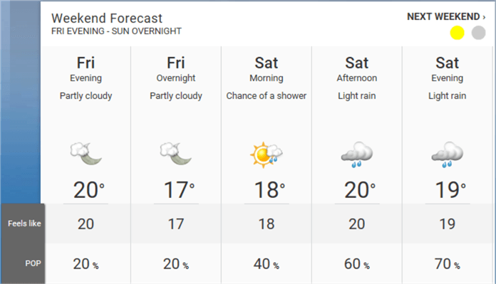
Figure 1 Weekend Forecast in Chicago, IL Updated on Thu Aug 29 6:45 PM [8]
We live in a world of uncertainty [9], not knowing the outcomes of a situation until it happens. Fortunately, we can use probability theory to measure and manage uncertainties. A probability, taking a value between 0 and 1, inclusively, reflects the chance or likelihood that an event will occur. The closer the probability is to 0, the less likely the event will occur. The closer the probability is to 1, the more likely the event will occur. Probabilities can be expressed as proportions that range from 0 to 1, or as percentages ranging from 0% to 100%. Thus, the statement that POP is 40% means there is a 40 percent chance that rain will occur at any given point in Chicago [7].
1.1 Basic Concepts
I have already used some statistics jargon when I introduced the definition of probability. We will frequently use them going forward. Let’s review these terms:
- Experiment: An activity that produces uncertain results. An example is tossing a coin.
- Outcome: A result of an experiment. An example is getting a head when tossing a fair coin.
- Sample space: The sample space, denoted as S, of an experiment is the set of all possible outcomes of the experiment. In the tossing a fair coin experiment, the sample space is {head, tail}. In general, an outcome in sample space can not further be divided into more elementary kinds of outcomes.
- Event: One or more outcomes of an experiment, which are a subset of the sample space. For example, in tossing a coin experiment, getting a head is an event, denoted as Event A. Getting a head or tail is also an event, denoted as Event B, for example. We say an event occurred when the actual outcome is in the subset.
We can visualize these concepts as Pebble World [10], shown in Figure 2. The sample space of the tossing a fair coin experiment is finite and it only includes two possible outcomes, head and tail, represented by two pebbles with the same mass. When a coin is considered "fair," it means that the chance of getting a head or a tail is equally likely. Event A is made up of the head outcome. Event B is made up of all possible outcomes.
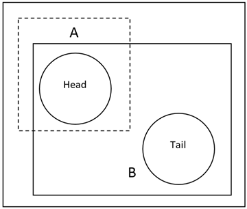
Figure 2 The sample space of the tossing a fair coin experiment
The two events illustrated in Figure 2 overlapped. To facilitate the understanding of probability, let’s study the relationship between events. We can graphically represent the relationship through Venn diagrams, named after their developer, John Venn. The Venn diagram starts with an enclosed area that represents the sample space. Next, the enclosed area is partitioned into parts that represent events. The R package "VennDiagram" [11] provides functions to construct Venn diagrams.
- Mutually Exclusive Events: Two events are mutually exclusive if they cannot occur at the same time during an experiment. Let’s design an experiment where we flip a fair coin. Let Event H be head and Event T be tail. We cannot get a "Head" and a "Tail" simultaneously when we flip the fair coin. The rectangle area in Figure 3 represents sample space and two circular areas represent two mutually exclusive events, respectively.
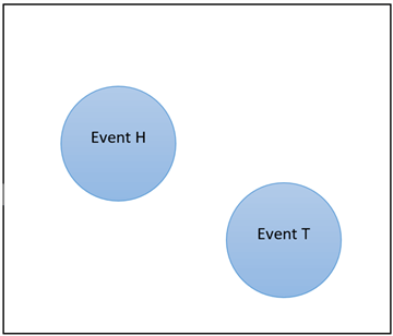
Figure 3 Venn Diagram: Mutually Exclusive Events
- Complementary Events:
The complement to Event A, denoted as
 , is a subset in the sample space that each outcome in the subset is not part
of Event A. In the tossing a fair coin experiment, for example, if we define
Event H is to flip a coin head, the complement of Event H is
 ,
which represents all other outcomes, shown in Figure 4.
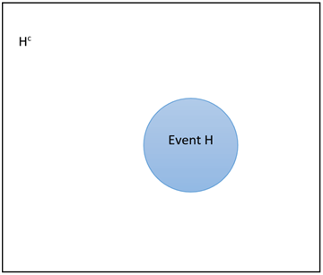
Figure 4 Venn Diagram: Complementary Events
- Union of Events: The union of Event A and B represents
all the instance where either Event A or Event B or both occur [12]. The
union of Event A and B is denoted as
 .
Let A be the event that students enrolled in Statistics class and B be the event
that students enrolled in Finance class. We assume these two classes are in
different class schedule.
  includes all students who either enrolled in Statistics class or Finance class
or both. Figure 5 illustrates
  ,
and the union is represented by the shaded area. The diagram also demonstrates
that events in the union may be mutually exclusive, like B and C, or they may
overlap, like A and B.
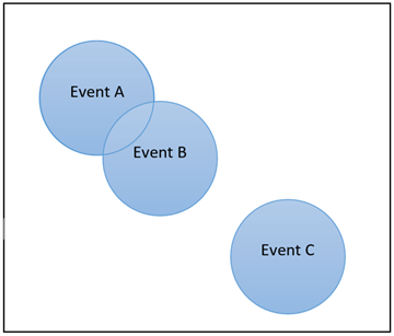
Figure 5 Venn Diagram: Union of Events
- Intersection of Events:
The intersection of Event A and B represents all the instance where both Event
A and Event B occur at the same time [12]. The intersection of Event A and B
is denoted as
 . In the
previous example, only students in both Statistics and Finance classes are part
of the intersection of the events. Figure 6 illustrates
  ,
and the intersection is represented by the shaded area.
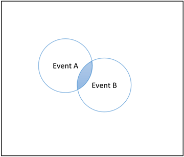
Figure 6 Venn Diagram: Intersection of Events
1.2 Three Main Methods of Measuring Probability
In the tossing a fair coin experiment, it is a common sense that we have 50% of chance to get a head. However, when we toss a weighted coin, the chance to get a head is not obvious. Furthermore, we may want to know the chance of using this coin to buy a toy. For different probability questions, several different approaches: classical, empirical and subjective, are available for determining probabilities.
1.2.1 Classical Probability
Classical probability is the earliest definition of the probability of an event, and it was considered as a naïve definition of probability [10]. This definition assumes that the sample space is finite, and each outcome of the experiment is equally likely to occur. I adopted the equation in [10] to calculate a probability of an event A with a finite sample space S:

where P(A) is the probability that Event A will occur.
In the experiment of tossing a fair coin, the sample space is {Head, Tail}. Let A be the event that the coin comes up a head. Since it is a fair coin, the chance to flip a head or tail are equally likely, thus we can apply the naïve definition:

Similarly, the experiment of tossing a fair coin twice has 4 possible outcomes: HH, HT, TH, and TT, where HH means that the coin comes up a head at the first time and comes up a tail at the second time. Let B be the event that the coin comes up a head at least once. This event is made up of 3 possible outcomes: HH, HT, and TH. By the naïve definition, we can compute the possibility of this event:

In order to use naïve definition, we must comprehend the experiment. Each outcome of the experiment should be equally likely to occur, and the total number of possible outcomes in the sample space should be finite. We are able to correctly count the number of outcomes associated to the event. To strengthen the understanding of naïve definition, let’s look at the airplane probability problem.
Example 1.2.1 (The Airplane Probability Problem) 100 passengers lined up to board an airplane with exactly 100 seats. Everyone has a ticket with an assigned seat number. However, the first passenger in line decides to sit in a randomly chosen seat. Every subsequent passenger takes his or her assigned seat. If the seat is taken by the other passenger, the passenger randomly takes an unoccupied seat. What is the probability that the last passenger in line gets to sit in his or her assigned seat?
Solution
To simplify the problem, we use sequential numbers, from 1 to 100, as seat numbers
in the airplane. Generally, the
 passenger takes the seat number
 .
The seat number of the last passenger is 100. When a passenger’s seat is taken
by the other passenger, all unoccupied seats are equally likely for him or her to
take.
First, we must understand the underlying experiment. Since the last passenger, the 100th passenger, is the last one to board to the airplane, any seat available to him or her should be available to previous 99 passengers. The first passenger takes a seat randomly, but other 98 sequential passengers will take their own seats when these seats are not occupied. So, there is no chance that seat numbers from 2 to 99 are available to the last passengers. If seat 49 is available to the last passenger, for example, certainly it will be available to the 49th passenger. When the seat 49 is available to the 49th passenger, the passenger takes this seat. Only two seats, seat 1 and seat 100, are available to the last passengers.
Next, to apply the naïve definition, we must ensure each outcome of the
experiment is equally likely to occur. In the boarding process, if anyone in the
first 99 passengers randomly take seat 1, seat 100 will be available to the last
passenger. Similarly, if anyone in the first 99 passengers randomly take seat 100,
seat 1 will be available to the last passenger. In the first 99 passengers, there
is one passenger, named passenger
 , who determines which seat left for the last passenger. The passenger
 views these two seats symmetrically. He or she has an equal chance to choose a seat
between seat 1 and seat 100. Thus, Seat 1 and seat 100 are equally likely to be
available to the last passenger.
Finally, we know the sample space is {seat 1, seat 100}. The total number of possible outcomes in the sample space is 2. Let event A be the last passenger takes the seat 100. Then, we know the number of outcomes associated to the event is 1. By the naïve definition, the probability that the last passenger in line gets to sit in his or her assigned seat is 50%.

By the way, this is a very interesting probability puzzle. Many people posted their solutions online. Arthur Breitman provided a simpler solution as a comment to Brett Berry’s solution [13].
Simulation:
A beautiful aspect of probability is that we can study problem via simulation [10]. We can run a simulation to verify our answers. To check the answer to the airplane probability puzzle, we can perform 10,000 simulations of boarding the airplane and examine the frequency of the fact that the seat 100 is available to the last passenger.
#----------------------------------------------------#
#    The Airplane Probability Puzzle Simulation      #
#----------------------------------------------------#
#Use defined function to find the available seat for the last passenger
seat.available.for.last.pax <- function(number.of.seats.on.plane) {
    #Each passenger has an assigned seat
    pax.assigned.seats <- seq(1:number.of.seats.on.plane)
    #The seat taken by each passenger is unknown
    pax.taken.seats <- rep(0, number.of.seats.on.plane)
    #All seats are available for the first passenger
    available.seats <- seq(1:number.of.seats.on.plane)
    #The first passenger boards airplane and randomly takes a seat
    pax.taken.seats[1] <- sample(available.seats, 1)
    #Every subsequent passenger takes his or her assigned seat if available,
    #and otherwise randomly takes a seat.
    for (i in pax.assigned.seats[c(-1, - number.of.seats.on.plane)]) {
        #Check if his/her seat was taken
        seat.is.taken <- which(pax.taken.seats == i)
        if (length(seat.is.taken) > 0) {
            #Find all available seats
            available.seats <- pax.assigned.seats[-pax.taken.seats]
            # Randomly Takes a seat
            pax.taken.seats[i] <- sample(available.seats, 1)
        }
        else {
            #Takes his or her assigned seat
            pax.taken.seats[i] <- i
        }
    }
    #Return the available seat
    return(pax.assigned.seats[-pax.taken.seats])
}

#Initialize variables
sim.outcome <- vector()
nsim <- 10000
number.of.seats.in.plane <- 100
#Start simulation
for (loop.count in 1:nsim) {
    #Invoking the function
    available.seats <- seat.available.for.last.pax(number.of.seats.in.plane)
    sim.outcome <- c(sim.outcome, available.seats)
}
#Summarize the simulation outcomes
table(sim.outcome)
The output of this program, shown in the follows, indicates that the probability of the last passenger taking his or her assigned seat is 49.93%. The simulation result is approximately equal to the computed answer. By the way, David Robinson posted an efficient simulation in his blog: The "lost boarding pass" puzzle: efficient simulation in R.
Sim.outcome
 1      100
5007   4993
1.2.2 Empirical Probability
A critical assumption in the classical approach (or naïve definition) is that each outcome in the sample space should be equally likely to occur. We should use a different way to determine probability when this assumption is violated. The other method is empirical probability, which is based on actual observations or available evidences. We also call this approach a relative frequency approach or a long-run relative frequency approach since we compute the probability from a relative frequency distribution:

In the experiment of tossing a coin, the two outcomes, head and tail, may not be equally likely to occur. Thus, the probability of event A, getting a head, may not be 50%. We can toss the coin again and again and keep track of the outcomes by counting heads and total tosses. Assuming we tossed coin 1000 times and got 296 heads, the long-run probability of getting a head would be:

This is a long-run experiment because we have repeatedly tossed the coin 1000 times. Alternatively, we can use existing evidences to compute a probability. For example, we can determine probability of an event on basis of historical data in a SQL server database. First, we run the following SQL script to read the relative frequencies of customer income in the "AdventureWorksDW2017" [14] database.
declare @total_count money

select @total_count = COUNT(*) * 1.0
  from [AdventureWorksDW2017].[dbo].[DimCustomer]

select
     concat(interval_floor, ' to under ', interval_ceiling) as [Class interval]
    ,count(*) as [Class frequencies]
,FORMAT(count(*)*1.0/@total_count,'0.###') as [Relative frequencies]
from (
       select
              floor([YearlyIncome]/20000.0)*20000 as interval_floor,
              floor([YearlyIncome]/20000.0)*20000 + 20000 as interval_ceiling
       from [AdventureWorksDW2017].[dbo].[DimCustomer]
) a
group by interval_floor, concat(interval_floor, ' to under ', interval_ceiling)
order by interval_floor;
The query results revealed that customer incomes were grouped into 9 classes, shown in Table 1. This table shows that 4054 customers are in the $20,000–$40,000 annual income range, and 206 customers are in the $160,000–$180,000 annual income range.
| Class interval | Class frequencies | Relative frequencies |
|---|---|---|
| 0 to under 20000 | 1155 | 0.062 |
| 20000 to under 40000 | 4054 | 0.219 |
| 40000 to under 60000 | 3417 | 0.185 |
| 60000 to under 80000 | 5476 | 0.296 |
| 80000 to under 100000 | 2184 | 0.118 |
| 100000 to under 120000 | 1045 | 0.057 |
| 120000 to under 140000 | 844 | 0.046 |
| 140000 to under 160000 | 103 | 0.006 |
| 160000 to under 180000 | 206 | 0.011 |
Table 1 Customer Income Frequency Distribution
The table also shows the proportion of customers in different income classes. If customers are equally likely distributed in each class, we can use classical method to determine the probability, that is, the chance of a customer in the $20,000–$40,000 annual income range should be 1/9, or 11.1%. The historical data in the database demonstrated that customers have not been evenly distributed in all classes, thus we cannot apply the naïve definition. In this case, the relative frequency approach was used, and the empirical probability of a random customer in the $20,000–$40,000 annual income range is 21.9%.
1.2.3 Subjective Probability
Under certain circumstances, both classical and empirical probability computation approaches do not fit. For example, how can I establish the probability that you will completely read this tip? When a strict counting-based approach seems unworkable, we may rely on experience and intuition to estimate the probabilities. This less structured and less formal approach to determine probability is called as a subjective approach.
To find the probability that you will completely read this tip, I use my personal estimate of the chance that the event will occur. On basis of my personal experience with similar situations, I would say that the chance you will complete reading this tip is 89%. It is possible the estimate can vary greatly from person to person. Due to this fact, not every statistician is comfortable with subjective probabilities [5].
1.3 General Definition of Probability
We have already defined the concept of probability and demonstrated three approaches to measure the uncertainty. To generalize the notion of probability, we adopted the definition in [10]:
A probability space consists of a sample space S and a probability function P
which takes an event  as input and returns P(A), a real number between 0 and 1 inclusively, as output.
The function P must satisfy the following axioms:
-

- If
 …
are mutually exclusive events, then

Any function P that satisfy these two axioms can be considered a valid probability. [10] also introduces how to interpret probability from two perspectives:
- The frequentist view: the probability represents a long-run frequency in which an event occurs over the total number of observations.
- The Bayesian view: the probability communicates a degree of uncertainty about the event in question.
2 - The Basic Rules of Probability
As an application of classical probability, we consider the birthday problem, which asks what is the probability that at least two persons in a group have the same birthday. We assume each person’s birthday is equally likely to be any of the 365 days of the year except February 29. Another assumption is that person’s birthdays are independent [10]. For the sake of simplicity, we assume the group size is 23.
By assumptions, each person’s birthday in the 23-person group is equally
likely to be any of the 365 days of the year. Therefore, person’s birthdays
can be arranged in
 ways. According to the classical probability definition, we should count the number
of occurrences that at least two person’s birthdays are same. However, this
counting is a challenge. To solve the birthday problem, we can use some basic rules
to simplify the puzzle.
2.1 Multiplication Rule for Mutually Independent Events
Given two mutually independent experiments A and B, the experiment A has
 possible outcomes, and the experiment B has
 possible outcomes. The total possible outcomes that both experiments A and B occur
is
 .
The following tree diagram demonstrates all possible outcomes of tossing a coin
two times:
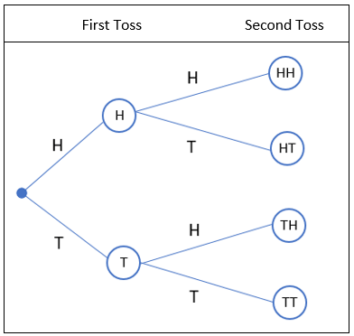
The first toss has two possible outcomes: H (for "head") and T (for "tail").
Since the second toss is independent on the first toss, for each possible outcome
of the first toss, the second toss has the two outcomes. Thus, total possible outcomes
are HH, HT, TH and TT. The number of total outcomes is
 .
.
The probability of an event is usually denoted by the symbol P(event), for example, P (2 heads). According to the definition, an event, for example event A, represent a group of outcomes from an experiment. To find the probability of two mutually independent events occurring together, we multiply the probability of the first event by the probability of the second event:

where A and B are mutually independent events. Thus, the possibility of 2-heads
occurrence is
 .
This rule applies to any number of mutually independent events.
Example 2.1.1 (Monty Hall problem) Suppose you're on a game show, and you're given the choice of three doors. Behind one door is a car, and behind others are goats. You pick a door, say #1, and the host, who knows what's behind the doors, opens another door, say #3, which a goat shows up. He says to you, "Do you want to pick door #2?" Is it to your advantage to switch your choice of doors? [15]
Solution
We have already known only one car is behind a door. Behind other two doors are goats. When the player does not switch his or her choice of doors after first selection, the player has 1/3 chance of winning the car. No matter which door the player picks, there is at least one goat behind a door. Then, the host shows the player a door with a goat. The host’s activity does not increase the chance of winning.
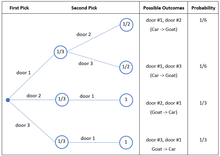
Let’s look at the scenario when the player decides to switch doors. We need to determine the probability that a car is behind the new selected door, which has not been opened by the host. We can use tree diagram to demonstrate the process. Due to the symmetry, we assume the car is behind door #1. If the car is behind other doors, for example door #2, we just label the door #2 as door #1.
As shown in the following tree diagram, there are 3 possible outcomes, door #1, door #2 and door #3, in the first selection. When door #1 was selected, the host would randomly open either door #2 or door #3 because two goats are behind these doors. Thus, the probability of the event "doors #1 and #2" is (1/3) *(1/2) = 1/6, and the probability of the event "doors #1 and #3" is (1/3) *(1/2) = 1/6.
When the player picked door #2 first time, the host must open door #3 because the goat is behind the door #3 and the car is behind door #1. Then, the player switches the door #1 and wins a car. The player also wins a car when he or she picks door #3 first time. The tree diagram reveals that switching gets the car 2/3 of the time.
Simulation
To check the answer to the Monty Hall problem, we can perform 10,000 simulations of playing the game and examine the frequency of the fact that the player wins the car.
#---------------------------------------------------#
#   The Monty Hall Problem Simulation               #
#---------------------------------------------------#

# Use defined function to find whether the player wins the car
monty.hall.simulation <- function(strategy) {
    # Initialize the return value
    rtnValue <- 0
    # Create three doors
    doors <- 1:3
    # Randomly hide a car behind a door
    cardoor <- sample(doors, 1)

    # The player randomly chooses a door
    chosen <- sample(doors, 1)
    if (strategy == "switch") {
        if (cardoor == chosen) {
            # If the door with a car behind was chosen,
            #the host randomly choose a door from the other two
            monty.door <- sample(doors[-chosen], 1)
        }
        else {
            # If the door with a car behind was not chosen,
            #the host must choose the door with a goat behind
            monty.door <- doors[-c(chosen, cardoor)]
        }
        # After the host open the door, the player picks the rest.
        chosen.2 <- doors[-c(chosen, monty.door)]
    }
    else {
        # The player does not switch
        chosen.2 = chosen
    }
    if (chosen.2 == cardoor) {
        rtnValue <- 1
    }
    return(rtnValue)
}

# Main Program
# Initialize variables
nsim <- 10000
sim.outcome.stay <- vector()
sim.outcome.switch <- vector()
# Start simulation
for (loop.count in 1:nsim) {
    # invoking the function
    is.win.stay <- monty.hall.simulation("stay")
    sim.outcome.stay <- c(sim.outcome.stay, is.win.stay)
    is.win.switch <- monty.hall.simulation("switch")
    sim.outcome.switch <- c(sim.outcome.switch, is.win.switch)
}
# Summarize the simulation outcomes
table(sim.outcome.stay)
table(sim.outcome.switch)
The output of this program, shown in the follows, indicates that the probability of wining a car is 33.7% when the player does not change the first selection after the host opens a door. The probability increases to 66.9% when the switching strategy is employed. The simulation result is close to the computed answer.
sim.outcome.stay
  0      1
6629   3371

sim.outcome.switch
  0      1
3306   6694
2.2 Addition Rule of Probabilities
An addition of two events, for example event A and event B, represents a combination
of two groups of outcomes. We may interpret the addition of two events by using
"either/or"
statement, for example, the likelihood of either event A happens, or event B happens.
When event A and event B are mutually exclusive, their corresponding groups do not
overlap. The general definition of probability states that the probability of event
 occurs is sum of their individual probabilities of occurrence. This rule can be
denoted by:

where A and B are mutually exclusive events. When event A and event B are not mutually exclusive, their corresponding groups overlap. Some outcomes belong to both event A and event B. If we simply add event A and event B together, we count each probability twice for these overlapped outcomes. We should make an adjusting for overcounting; thus, the general rule of addition can be denoted by:

This is a special case of inclusion-exclusion, which finds the probability of
a union of events [10]. In general, for any events
 ,
,

The chapter 4 in the book [10] proved inclusion- exclusion for n>2. To demonstrate the application of inclusion-exclusion, let’s look at the de Montmort’s matching problem.
Example 2.2.1 (de Montmort’s matching problem) There are N cards, labeled 1 through N, in a deck. What is the probability of the number on the card matching the card’s position in the deck?
Solution
A well-shuffled deck of
 cards has
 possible orderings. All these possible orderings construct the sample space of the
experiment. Let
 be the event that the number on the card
 matches the
 position in the deck. Thus, we should sum up these individual probabilities of occurrences,
which is the probability of union
 .
.
Since every card has an equal chance in a position in the deck, we can apply the classical probability method:

Let
 be the event that the number on the card
 matches the
 position in the deck, where
 .
When events
 and
and
 both occurred, that meant the card
 is at the position
 and card
 is at the position
 .
And other (n-2) cards can be in any positions. Thus, the probability of both events
occurring at the same time is computed through:

In general, the probability of all
 events occurring at the same time is computed by:

So far, we have picked up one group of
 events and then find the probability of all
 events occurring at the same time. Since there are
 events in total, there are
 possible ways to pick up
 events. The item in the inclusion-exclusion formula corresponding to the
 events occur at the same time is obtained by:

where
 represent
 individual events occur at the same time. It is always a good practice to validate
an equation with some extreme cases. The equation can correctly represent the items
in the inclusion-exclusion formula when
 1 and n. Substitute these terms in the inclusion-exclusion formula, we have obtained
the probability:

When
 is very large, the probability is close to
 .
.
Simulation
To check the answer to the de Montmort’s matching problem, we can perform 10,000 simulations of playing the game and examine the frequency of the fact that the match occurs.
#---------------------------------------------------#
#   The de Montmorts Matching Problem Simulation    #
#---------------------------------------------------#

# Use defined function to observe at least one match
observe.at.least.one.match <- function(cards.in.deck) {
    # Initialize the return value
    rtnValue <- 0
    # The position numbers of cards in the deck
    position.number <- 1:length(cards.in.deck)
    # Find whether at least one card matches the position number
    total.matches <- sum(position.number == cards.in.deck)
    if (total.matches > 0) {
        rtnValue <- 1
    }
    return(rtnValue)
}

# Main Program
# Initialize variables
N <- 100
nsim <- 10000
sim.outcome <- vector()
# Start simulation
for (loop.count in 1:nsim) {
    # Generate N cards in a random order
    cards <- sample(1:N)
    # Invoking the function
    is.match <- observe.at.least.one.match(cards)
    sim.outcome <- c(sim.outcome, is.match)
}
# Summarize the simulation outcomes
table(sim.outcome)
The output of this program, shown in the following, indicates that the probability of observing at least one match is 63.32%. The simulation result is close to the computed answer.
sim.outcome
 0      1
3668   6332
2.3 Complement Rule of Probabilities
In the sample space
 ,
all outcomes not being included in a given event subset, for example event
 ,
comprise the complement of that subset,
 .
Then, we know
 ,
therefore
 .
In the rolling one die experiment, let event A be 4 spots. Then probability of event
A happening is 1/6, and the probability of A not happening must be 5/6. On basis
of the axioms given in section 1.3, we have known these axioms:


Then, we have obtained the complement rule of probabilities:

The complement rule seems obvious and simple, but it is a good strategy to simplify complicated problems. Sometimes, it is easier to find the probability of a complement of an event. Let’s revisit the birthday problem:
Example 2.3.1 (Birthday problem) There are 23 persons in a room. We assume each person’s birthday is equally likely to be any of the 365 days of the year except February 29. In addition, we also assume person’s birthdays are independent. What is the probability that at least two persons in a group have the same birthday?
Solution: To solve a probability problem, it is always a good
strategy to use an extreme scenario to understand the problem and validate the solution.
Let’s find out what is the probability 2 persons share the same birthday.
Since each person can be born on any day of a year, there are
 ways to assign birthdays to these 2 persons, and the first person can be any day
in a year. But when we consider the second person should have the same birthday
day as the first person, there are
 ways to assign birthdays to these 2 persons. Thus, the probability can be computed
by the naïve definition:

The counting problem becomes hard when more than 2 persons are involved in the calculation. Instead of computing the probability that at least 2 persons share a birthday, we compute the probability of the complement that no people share a birthday. We have known this equation:

In a room of 23 persons, no people share a birthday. This indicates that everyone was born on a different day. The number of permutations of 365 days taking 23 at a time is given by:

Since the total amount of arranging birthday is
 ,
we compute the probability through the naïve definition:

Therefore

Many people are surprised to find that, within a group of 23 persons, there is a 50.7% chance that at least two persons were born on the same day.
Simulation
To check the answer to the Birthday problem, we can perform 10,000 simulations that randomly assign birthdays to 23 persons. Then we examine the frequency of the fact that the birthday match occurs.
#---------------------------------------------------#
#   The Birthday Problem Simulation                 #
#---------------------------------------------------#

# Use defined function to find at least one match
birthday.simulation <- function(group.size) {
    # Initialize the return value
    rtnValue <- 0
    # Randomly assign a birthday to each person
    birthdays <- sample(1:365, group.size, replace = TRUE)
    # Use duplicated function to detect whether there is a match
    if (sum(duplicated(birthdays)) > 0) {
        # Detect there is at least one match
        rtnValue <- 1
    }

    return(rtnValue)
}

# Main Program
# Initizlize variables
nsim <- 10000
sim.outcome <- vector()
# Start simulation
for (loop.count in 1:nsim) {
    # Invoking the function
    at.least.a.match <- birthday.simulation(23)
    sim.outcome <- c(sim.outcome, at.least.a.match)
}
#Summarize the simulation outcomes
table(sim.outcome)
The output of this program, shown in the follows, indicates that the probability of at least 2 persons sharing a birthday is 50.5%. The simulation result is close to the computed answer.
sim.outcome
 0      1
4950   5050
2.4 Conditional Probability
Conditioning is the soul of statistics [10]. The conditional probability, denoted
by
 ,
is the probability of the occurrence of one event, for example
 ,
given that some other event has already occurred or will occur. We write the definition
in these equations:

For example, we look at the experiment of rolling a pair of colored dice: one red die and one black die. Let A be the event that the red die shows 6 spots, and B be the event that the pair of dice shows 9 spots. According to the naïve definition, we know probabilities of these events:


Given the evidence that the pair of dice show 9 spots, that is, the event B occurred, we can update the probability that the red die shows 6 spots:

This example demonstrated a process to incorporate evidence into our understanding
and then update our belief.
 is called the prior probability of A, and
 is called the posterior probability of A.
Section 2.1 gave the special rule of multination for mutually independent events. From the definition of conditional probability, we can draw the general rule of multiplication:

Furthermore, we derived the following equation, which is known as Bayes’
rule. With the Bayes’ rule, we can calculate
 from information about
 (or vice versa). This makes this rule extremely famous and extremely useful [10].

Example 2.4.1 (Market Basket Analysis) Frequent pattern mining, which detects recurring relationships in a data set, is a function of data mining. An association rule can be used to represent the pattern, for example:

where the rule support measures the percent of sales transactions that customers purchased bike and helmets together, and the rule of confidence measures the percent of customers who bought a bike also bought a helmet. Let’s discover such an association rule in the "AdventureWorks2017" [14] database.
Solution: Let "Bike" be the event that a customer purchased a bike and let "Helmet" be the event that a customer purchased a helmet. Thus, rule support and confidence, two measures of rule interestingness, are represented by the following equations:


To find support and confidence, we need to know the total amount of transactions, total amount of transactions that both a bike and a helmet were ordered, and total amount of transactions that a bike was ordered. Then, we can obtain these two measures by:


where
 is computed by the empirical method:

We used the following T-SQL scripts to discover the association rule:
declare @total_transactions money
declare @total_transactions_bikes money
declare @total_transactions_bikes_and_helmets money

SELECT @total_transactions = COUNT(DISTINCT h.[SalesOrderID])
FROM [Sales].[SalesOrderHeader] h INNER JOIN [Sales].[Customer] b
on b.[CustomerID] = h.CustomerID
WHERE b.PersonID is not null

SELECT @total_transactions_bikes = COUNT(DISTINCT h.[SalesOrderID])
FROM [Sales].[SalesOrderDetail] d
INNER JOIN [Sales].[SalesOrderHeader] h on d.SalesOrderID = h.SalesOrderID
INNER JOIN [Sales].[Customer] b on b.[CustomerID] = h.CustomerID
INNER JOIN [Production].[Product] p on d.ProductID = p.ProductID
INNER JOIN [Production].[ProductSubcategory] s on p.ProductSubcategoryID = s.ProductCategoryID
INNER JOIN [Production].[ProductCategory] c on s.ProductCategoryID = c.ProductCategoryID
WHERE b.PersonID is not null
AND c.[Name] = 'Bikes'

SELECT @total_transactions_bikes_and_helmets = COUNT(DISTINCT h.[SalesOrderID])
FROM [Sales].[SalesOrderHeader] h
INNER JOIN [Sales].[Customer] b on b.[CustomerID] = h.CustomerID
INNER JOIN [Sales].[SalesOrderDetail] d1 on d1.SalesOrderID = h.SalesOrderID
INNER JOIN [Production].[Product] p on d1.ProductID = p.ProductID
INNER JOIN [Production].[ProductSubcategory] s1 on p.ProductSubcategoryID = s1.ProductCategoryID
INNER JOIN [Production].[ProductCategory] c1 on s1.ProductCategoryID = c1.ProductCategoryID
INNER JOIN [Sales].[SalesOrderDetail] d2 on d2.SalesOrderID = h.SalesOrderID
INNER JOIN [Production].[Product] p2 on d2.ProductID = p2.ProductID
INNER JOIN [Production].[ProductSubcategory] s2 on s2.ProductCategoryID = p2.ProductSubcategoryID
WHERE b.PersonID is not null
AND c1.[Name] = 'Bikes' and s2.[Name] = 'Helmets'

select r.P_bike, r.P_bike_and_helmet, (r.P_bike_and_helmet/r.P_bike) as P_helmet_given_bike
from
(
  select (@total_transactions_bikes /@total_transactions) as P_bike
  ,(@total_transactions_bikes_and_helmets / @total_transactions) as P_bike_and_helmet
) r
The query result, shown in the following, indicates that the probability of purchasing a bike is 19.65%, the probability of purchasing a bike and a helmet is 1.75% and the probability of purchasing a helmet given purchasing a bike is 8.9%.
P_bike   P_bike_and_helmet   P_helmet_given_bike
0.1965   0.0175              0.089
On basis of the SQL result, we obtained these two measures:


A support of 1.75% means that 1.75% of sales transactions under analysis show that bike and helmet are bought together. A confidence of 8.9% means that 8.9% of the customers who bought a bike also bought a helmet. However, this association rule may not be considered interesting because the value of confidence is low. Typically, users set a minimum support threshold and a minimum confidence threshold. Association rules are considered interesting if they satisfy these two thresholds [16].
Summary
To really discover knowledge from huge amount of data, we should not only know how to use the tools, but also understand these principles underlying them. Probability theory is the mathematical foundation for statistical inference, and thus essential for data science practice.
This tip has discussed what the concept of probability is, and how to apply basic probability principals to solve some famous probability puzzles. First, the tip studied the naïve definition of probability, then studied the general definition of probability. Venn diagrams were used to illustrate some core probability concepts. Next, we have discussed four basic rules of probability: the multiplication rule, the addition rule, the complement rule and the conditional probability. We used tree diagrams to effectively demonstrate the multiplication rule. We also derive Bayes’ rule from the definition of conditional probability.
References
[1] Dyche, J. (2015). The New IT: How Technology Leaders are Enabling Business Strategy in the Digital Age. New York, NY: McGraw-Hill.
[2] Han, J., Kamber, M., & Pei, J. (2011). Data Mining: Concepts and Techniques (3rd Edition). Waltham, MA: Morgan Kaufmann.
[3] Zhou, N. (2018, November 11). Getting Started with Data Analysis on the Microsoft Platform - Examining Data. Retrieved from https://www.mssqltips.com/sqlservertip/5758/getting-started-with-data-analysis-on-the-microsoft-platform--examining-data/.
[4] Zhou, N. (2019, May 28). Numerically Describing Dispersion of a Data Set with SQL Server and R. Retrieved from https://www.mssqltips.com/sqlservertip/6058/numerically-describing-dispersion-of-a-data-set-with-sql-server-and-r/.
[5] Bergquist, T., Jones, S., & Freed, N. (2013). Understanding Business Statistics. Hoboken, NJ: John Wiley & Sons.
[6] Hummelbrunner, S. A., Rak, L. J., Fortura, P., & Taylor, P. (2003). Contemporary Business Statistics with Canadian Applications (3rd Edition). Toronto, ON: Prentice Hall.
[7] theweathernetwork.com (2019). Probability of Precipitation. Retrieved from https://www.weather.gov/ffc/pop.
[8] theweathernetwork.com (2019). Weekend Forecast. Retrieved from https://www.theweathernetwork.com/us/weekend-weather-forecast/illinois/chicago/.
[9] McEvoy, M. D. (2018). A Guide to Business Statistics. Hoboken, NJ: John Wiley & Sons.
[10] Hwang, J. & Blitzstein, K. J. (2015). Introduction to Probability. Boca Raton, FL: CRC Press.
[11] Chen, H. (2018, March 28). VennDiagram: Generate High-Resolution Venn and Euler Plots. Retrieved from https://cran.r-project.org/web/packages/VennDiagram/index.html.
[12] Abdel-Raouf, F. & Donnelly, A. R. (2016). Statistics (3rd Edition). Indianapolis, IN: Alpha.
[13] Berry, B. (2017). The Airplane Probability Problem. Retrieved from https://medium.com/i-math/solving-an-advanced-probability-problem-with-virtually-no-math-5750707885f1.
[14] Kess, B. (2017, December 12). AdventureWorks sample databases. Retrieved from https://github.com/Microsoft/sql-server-samples/releases/tag/adventureworks/.
[15] Savant, V. M. (1990). "Ask Marilyn" by Savant, Marilyn vos in Parade Magazine, 2 December 1990, p 25, and 17 February 1991, p 12.
[16] Kros, F. J. & Rosenthal A. D. (2015, December). Statistics for Health Care Management and Administration: Working with Excel (3th edition). San Francisco, CA: Jossey-Bass.
Next Steps
- There are some famous probability puzzles, for example, the airplane probability problem, the birthday problem, the de Montmort’s matching problem, and the Monty Hall problem. Many people have already provided solutions. You may see these puzzles in job interviews or math competitions. We should be able to work out these puzzles, or at least we should understand these solutions. To study probability in more depth, I strongly recommend the free course: Statistics 110: Probability, which has been taught at Harvard University by Professor Joe Blitzstein.
- Check out these related tips:
- Getting Started with Data Analysis on the Microsoft Platform - Examining Data
- Getting Started with Data Analysis and Visualization with SQL Server and R
- Numerically Describing Dispersion of a Data Set with SQL Server and R
- Exploratory Data Analysis with Python in SQL Server 2017
- Using SQL to Assess Goodness of Fit to Normal and Uniform Distributions
- SQL Server T-SQL Code to Generate A Normal Distribution
About the author
 Nai Biao Zhou is a Senior Software Developer with 20+ years of experience in software development, specializing in Data Warehousing, Business Intelligence, Data Mining and solution architecture design.
This author pledges the content of this article is based on professional experience and not AI generated.
View all my tips


