Problem
In my previous tip [1], I have characterized a numeric data set through measures of central tendency: the mean, the median and the mode. All values in the data set tend to cluster around these central values. We can feel and understand the data set through these statistical measures. Data differ in a data set. For example, customer yearly incomes in AdventureWorks sample database [2] varied from customer to customer. Business users may want to know how far individual customer’s yearly incomes have strayed from the mean. Measures of central tendency do not focus on the variability of the data in a data set. To obtain a more meaningful and accurate numerical description of a data set, business users want to understand how to describe the spread or the dispersion of a data set. In addition, the dispersion in a bivariate data set, illustrated by a scatter diagram, may reveal a strong association between the paired variables. Business users would like to know how to use a numeric value to describe the degree of the association.
Solution
The common measures of dispersion include the range, the interquartile range, the average deviation from the mean, the variance, the standard deviation, and the coefficient of variation [3]. To describe the association of two variables in a bivariate dataset, we are going to study two important measures of association: covariance and correlation coefficient. All these measures, in conjunction with measures of central tendency, can make possible a more complete numerical description of a data set.
We randomly selected 35 customers from the AdventureWorks sample database "AdventureWorksDW2017.bak" [2], then studied how customer yearly income data were spread out and how the customer income and age were related. Since the size of sample data set was 35, we were able to manually calculate all these measures.
The population data set, which includes yearly income and age data of all individual customers, is available in the database. We used “R Tools for Visual Studio (RTVS)”, introduced in my other tip “Getting Started with Data Analysis on the Microsoft Platform – Examining Data“, to compute these measures.
The solution was tested with SQL Server Management Studio V17.4, Microsoft Visual Studio Community 2017, Microsoft R Client 3.4.3, and Microsoft ML Server 9.3 on Windows 10 Home 10.0 <X64>. The DBMS is Microsoft SQL Server 2017 Enterprise Edition (64-bit).
1 – Population and Sample
1.1 Reviewing Basic Statistics Concepts
It’s been said that the easiest way to grow your customers is not to lose them. Business users want to discover valuable insight from existing customers and keep them coming back. To study AdventureWorks customers, we collected customer yearly income and age data. These customers, upon which the measurements are made, are called experimental units. These measured values of interest are termed observations. Yearly income and age, the properties of the experimental units being measured, are called variables.
A data set is collected for all AdventureWorks customers of interest is called a population. When we are interested in all customers in the AdventureWorks database, we obtain a finite population that consists of a limited and specifically known number of items. When we study all customers of AdventureWorks, including existing customers and future customers, due to unknown future customers, the population is an infinite population in which the number of items is unlimited or not specifically known. We use the term parameter to describe a characteristic of a population.
Due to physical constraints, time constraints, cost constraints, and test constraints [3], sometimes we cannot measure a population. Thus, we often have to select a portion of a population and to make inferences about the population parameters based on the information in the selected portion. The selected portion is called sample. The process to select the portion of the population is called sampling. The most common type of sampling procedure is to give every different sample of fixed size in the population an equal chance of selection. Such a sample is called a random sample, which is likely to be representative of the population [4]. We use the term statistic to describe a characteristic of a sample.
Descriptive statistics and inferential statistics are two major branches of statistics. Frequently, we use sample statistics to estimate population parameters. Business users can make important decisions on the basis of inferences made about the population through analyzing the sample data. Table 1 summarizes some differences between a population and a sample.
| Population | Sample | |
|---|---|---|
| Definition | A population data set is a collection (or set) of data measured on all experimental units of interest to you. | A sample is a subset of data selected from a population. |
| Term for all characteristics | Parameters, for example, population mean and population standard deviation. | Statistics, for example, sample mean and sample standard deviation. |
| Symbol for Mean | µ | |
| Symbol for Correlation Coefficient | ρ | |
| Symbol for Size | | n |
| Symbol for Standard Deviation |  |  |
Table 1 – Population versus Sample [3,4]
1.2 Preparing Data Sets
The population in this study is a set of all customers in the AdventureWorks database. The customer’s yearly income and the customer’s age are two variables of interest. The population can be obtained by the following SQL query:
SELECT [CustomerKey]
     ,[YearlyIncome]
     ,[Age]
 FROM [dbo].[vTargetMail]
The query returns a data set with 18,484 customers. The data set is too large to analyze without using modern computing technologies. Inferential statistical analysis, which is out scope of this tip, allows us to make inferences about the large data set by analyzing a small data set. We have prepared a sample data set by a random selection of 35 customers, shown in Table 2, from the population data set to demonstrate manual computation process. In this tip, we will study measures of dispersion on the population data set and the sample data set. Since we have no interest in customer key, this is a bivariate data set made up of two paired variables: yearly income and age. We will determine the range, the interquartile range, the average deviation from the mean, the variance, the standard deviation, and the coefficient of variation for the yearly income variable. We also study covariance and correlation between two variables.
| Customer Key | Yearly Income | Age | Customer Key | Yearly Income | Age | Customer Key | Yearly Income | Age | Customer Key | Yearly Income | Age |
|---|---|---|---|---|---|---|---|---|---|---|---|
| 17479 | 10000 | 64 | 17347 | 30000 | 35 | 20779 | 60000 | 48 | 26719 | 80000 | 53 |
| 18895 | 10000 | 58 | 25727 | 30000 | 51 | 28319 | 60000 | 42 | 15843 | 80000 | 44 |
| 23792 | 20000 | 58 | 23774 | 30000 | 42 | 26139 | 60000 | 46 | 13623 | 80000 | 40 |
| 25514 | 20000 | 37 | 17978 | 40000 | 44 | 13878 | 60000 | 45 | 12055 | 90000 | 44 |
| 13057 | 30000 | 38 | 12016 | 40000 | 37 | 23213 | 70000 | 45 | 29209 | 90000 | 42 |
| 13722 | 30000 | 58 | 16984 | 40000 | 43 | 25943 | 70000 | 34 | 18174 | 90000 | 58 |
| 18975 | 30000 | 63 | 28358 | 50000 | 48 | 17180 | 70000 | 59 | 11900 | 90000 | 38 |
| 22974 | 30000 | 76 | 26299 | 60000 | 35 | 11069 | 80000 | 52 | 13307 | 100000 | 78 |
| 17947 | 30000 | 54 | 16093 | 60000 | 47 | 17683 | 80000 | 39 |
Table 2 – Employee Sample Data
2 – The Range
The range is the simplest measures of dispersion and is a crude measure of variability. it is the difference between the highest and the lowest values in a data set. Some people use an ordered pair of smallest and largest numbers, like [smallest, largest], to denote the range of a data set. Except for some descriptive purpose, the range as a measure of variability is rarely used in statistical analysis applications [5].
When numeric values in a data set are arranged in ascending order, for example, the yearly income data in Table 2, the first value in the data set is the lowest value and the last is the highest one. Then, the range of the yearly income is simply the largest value minus the smallest value:
The lowest yearly income: 10,000
The highest yearly income: 100,000
The range: 100,000 – 10,000 = 90,000
The range is affected by extreme values; therefore, it may be misleading. For example, if we add an employee with yearly income 1,000,000 to the sample data set, the range increases to 990,000. The statement that customer yearly income is between 10,000 and 1,000,000 will mislead the audience, since all other customers make less than 100,000 a year.
Usually, it is impractical to manually arrange numeric values in a population data set in an ascending order. We can use R function, range (x, na.rm = FALSE), to find the range of a data set. We run the following R codes through RTVS:
library(RODBC)
# Load data from data warehouse
dbConnection <-'Driver={SQL Server};Server=.;Database=AdventureWorksDW2017;Trusted_Connection=yes'
channel <- odbcDriverConnect(dbConnection)
InputDataSet <- sqlQuery(channel,
'        SELECT[CustomerKey]
          , [YearlyIncome]
              , [Age]
          FROM [dbo].[vTargetMail]
'
)
# Read customer income data to a vector
customer_income <- InputDataSet$YearlyIncome
# Apply range function to calculate the range
income_range <- range(customer_income)
# Output the range
cat("The lowest yearly income:", format(income_range[1], big.mark =","),"\n")
cat("The highest yearly income:", format(income_range[2], big.mark =","),"\n")
cat("The range:", format(income_range[2] - income_range[1], big.mark =","),"\n")
The output of these R codes is shown in the R interactive window. The range of the yearly income in the population data set is 160,000.
The lowest yearly income: 10,000
The highest yearly income: 170,000
The range: 160,000
Table 3 shows the ranges of the customer yearly income variable for the population data set and the sample data set. The range of the population data set is almost twice as many as the range of the sample data set. That means the population data set contains some extreme values. This shows the limitation that range calculation relies on only two extreme values. No other values between these two extremes are involved in the range calculation.
| Population | Sample | |
|---|---|---|
| The lowest yearly income | 10,000 | 10,000 |
| The highest yearly income | 170,000 | 100,000 |
| The range | 160,000 | 90,000 |
Table 3 – The Ranges of Customer Yearly Income
3 – The Interquartile Range
The range where the middle 50% of the values lie is called interquartile range (IQR). IQR is especially useful to users who have more interests in values toward the middle and have less interests in extremes. In percentile terms, IQR is the distance between the 75th percentile and 25th percentile. The 75th percentile is located at the 3rd quartile, or Q3. The 25th percentile is located at the 1st quartile, or Q1. The IQR provides a clearer description of the overall data set by removing these extreme values in the data set. Thus, the IQR is more meaningful than the range.
My other tip “Getting Started with Data Analysis and Visualization with SQL Server and R” has studied the concept of quartile and manually calculated IQR for the customer total purchase amount data set. We are going to follow the same procedure to compute IQR for the customer yearly income variable:
Step 1: Find the position number of the 25th percentile.
Step 2: Find the value at the 9th position, which is 30,000.
Step 3: Find the position number of the 75th percentile.
Step 4: Find the value at the 27th position, which is 80,000.
Step 5: Compute IQR.
Therefore, the IQR of the yearly income variable for the sample data set is 50,000, which means the span of middle 50% of the yearly income data is 50,000.
We can use R functions IQR(x, na.rm = FALSE) and Quantile(x, na.rm = FALSE) to compute IQR and quantiles of the customer yearly income data for the population data set. We run the following R codes through RTVS:
library(RODBC)
# Load data from data warehouse
dbConnection <-'Driver={SQL Server};Server=.;Database=AdventureWorksDW2017;Trusted_Connection=yes'
channel <- odbcDriverConnect(dbConnection)
InputDataSet <- sqlQuery(channel,
'
        SELECT[CustomerKey]
              , [YearlyIncome]
              , [Age]
          FROM[dbo].[vTargetMail]
'
)
# Read customer income data to a vector
customer_income <- InputDataSet$YearlyIncome
# Apply IQR function to calculate the IQR
income_iqr <- IQR(customer_income)
# Apply quantile function to calculate quantiles
income_quantile <- quantile(customer_income)
# Output the range
cat("Q1:", format(income_quantile[2], big.mark =","),"\n")
cat("Q3:", format(income_quantile[4], big.mark =","),"\n")
cat("IQR:", format(income_iqr, big.mark =","),"\n")
The output of these R codes has been written in the R interactive window. The result indicates that the range of the middle 50% of the yearly income data for the population data set is 40,000.
Q1: 30,000
Q3: 70,000
IQR: 40,000
Table 4 shows Q1, Q3 and the IQR of customer yearly income data for the population data set and the sample data set. The IQR for the population data set is close to the one of the sample data set. Because the number of extreme values is reduced, the IQR is more meaningful than range to represent the dispersion of a data set.
| Population | Sample | |
|---|---|---|
| Q1 | 30,000 | 30,000 |
| Q3 | 70,000 | 80,000 |
| IQR | 40,000 | 50,000 |
Table 4 – The IQR and Quartiles
4 – The Average Deviation from the Mean
Both the range and the IQR use only use two values in a data set to represent a measure of dispersion. The average deviation from the mean of the data set considers all values in the data set. The deviation is the difference between the value of an observation in the data set and the mean of the data set. The average deviation from the mean is the average of the absolute deviation. The average deviation from mean for a sample data set can be determined by using the formula:
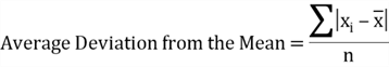
Where
![]()
![]()
![]()
To calculate the average deviation from mean for a population data set, we can use the formula [3]:

Where
![]()
![]()
![]()
The average yearly income of the sample data set is 54,286. Now we compute the absolute deviations ![]() by hand, as shown in Table 5. The average of
by hand, as shown in Table 5. The average of ![]() is 22,775. This means, on the average, the customer yearly incomes were 22,775 away from the mean 54,286.
is 22,775. This means, on the average, the customer yearly incomes were 22,775 away from the mean 54,286.
| Yearly Income | | Yearly Income | | Yearly Income | | Yearly Income | |
| 10000 | 44286 | 30000 | 24286 | 60000 | 5714 | 80000 | 25714 |
| 10000 | 44286 | 30000 | 24286 | 60000 | 5714 | 80000 | 25714 |
| 20000 | 34286 | 30000 | 24286 | 60000 | 5714 | 80000 | 25714 |
| 20000 | 34286 | 40000 | 14286 | 60000 | 5714 | 90000 | 35714 |
| 30000 | 24286 | 40000 | 14286 | 70000 | 15714 | 90000 | 35714 |
| 30000 | 24286 | 40000 | 14286 | 70000 | 15714 | 90000 | 35714 |
| 30000 | 24286 | 50000 | 4286 | 70000 | 15714 | 90000 | 35714 |
| 30000 | 24286 | 60000 | 5714 | 80000 | 25714 | 100000 | 45714 |
| 30000 | 24286 | 60000 | 5714 | 80000 | 25714 |
Table 5 – Employee Yearly Income Absolute Deviation
Calculating the average deviation from mean using the formula can be tedious and time consuming. Here comes R to help. We can use R functions mean(x, na.rm = FALSE) and abs(x) to compute the customer yearly income for the population data set. We run the following R codes through RTVS:
library(RODBC)
# Load data from data warehouse
dbConnection <-'Driver={SQL Server};Server=.;Database=AdventureWorksDW2017;Trusted_Connection=yes'
channel <- odbcDriverConnect(dbConnection)
InputDataSet <- sqlQuery(channel,
'
        SELECT[CustomerKey]
              , [YearlyIncome]
              , [Age]
          FROM[dbo] .[vTargetMail]
'
)
# Read customer yearly income data to a vector
customer_income <- InputDataSet$YearlyIncome
# Apply mean and abs functions to calculate the average deviation from the mean
income_mad <- mean(abs(customer_income - mean(customer_income)))
# Output the average deviation from the mean
cat("The average deviation from the mean :", format(income_mad, big.mark =","),"\n")
The R interactive window presents the output of these R codes. The result indicates that, on the average, the customer yearly incomes were 25,475 away from the population mean.
The average deviation from the mean: 25,474.97
Table 6 shows the average deviation from mean of customer yearly income in the population data set and the sample data set. The comparison demonstrated in Table 6 implies that the dispersion for the sample data set can be used as a representative of the dispersion for the population data set.
| Population | Sample | |
|---|---|---|
| Mean | 57,306 | 54,286 |
| The average deviation from the mean | 25,475 | 22,775 |
Table 6 – The Average Deviation from the Mean
5 – The Variance and Standard Deviation
The variance and standard deviation are widely used in statistics. The variance is the average of the squared deviations about the arithmetic mean for a data set, and the standard deviation is the positive square root of the variance. The formula for the population variance is shown as follows:
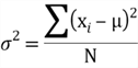
Where:
![]()
![]()
![]()
![]()
A sample is a subset of data selected from a population [4]. To make the sample variance a better estimate of the population variance, we use an unbiased estimator of the variance of the population. An unbiased estimator is a sample estimator of a population parameter for which the mean value from all possible samples is equal to the population parameter value [5]. We compute the sample variance by this formula:

Where:
![]()
![]()
![]()
![]()
The standard deviation, an especially important measure of dispersion, has the same unit as values in the data set. We can determine the minimum percentage of observations that fall within a given number of standard deviations from the mean, regardless of the shape of the distribution according to Chebyshev’s theorem [6]. Since absolution deviations ![]() have been obtained as shown in Table 5, we can obtain the standard deviation through the following steps:
have been obtained as shown in Table 5, we can obtain the standard deviation through the following steps:
Step 1: Square each absolution deviations;
Step 2: Sum all squared absolution deviations;
Step 3: Divide the sum by one fewer than the sample size. The result is the variance;
Step 4: Take the square root of the variance;

Chebyshev’s theorem [6] states that, for either a sample or a population, the percentage of observations that fall within k (for k >1) standard deviations of the mean will be at least
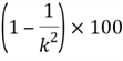
For the sample data set in Table 2, the sample mean of yearly income is 54,286 and standard deviation is 26,041. Let’s find the percentage of values that fall within 2 standard deviations of the mean (or k=2), which the interval is 54,286±2(26,041), or from 2,204 to 106,368. We obtain the percentage by using the following calculation:

Table 2 indicates 100% of income data fall within the interval. Chebyshev’s theorem predicted the minimum of 75%. The actual result agreed with the result from theorem.
R functions, var() and sd() are used to compute the sample variance and sample standard deviation, respectively. However, for large sample size, for example n≥30, the subtraction of 1 from n makes very little difference [6]. Therefore, we are going to calculate population variance and standard deviation by using these two functions as well.
library(RODBC)
# Load data from data warehouse
dbConnection <-'Driver={SQL Server};Server=.;Database=AdventureWorksDW2017;Trusted_Connection=yes'
channel <- odbcDriverConnect(dbConnection)
InputDataSet <- sqlQuery(channel,
'
        SELECT [CustomerKey]
              , [YearlyIncome]
              , [Age]
          FROM[dbo].[vTargetMail]
'
)
# Read customer yearly income data to a vector
customer_income <- InputDataSet$YearlyIncome
# Apply var function to calculate the population variance
income_var <- var(customer_income)
# Apply sd function to calculate the population standard deviation
income_std <- sd(customer_income)
# Output the average deviation from the mean
cat("The population variance:", format(income_var, big.mark =","),"\n")
cat("The population standard deviation:", format(income_std, big.mark =","),"\n")
We can find the calculation results in the R interactive window:
The population variance: 1,042,375,574
The population standard deviation: 32,285.84
Table 7 shows the variance and standard deviation of customer yearly income in the population data set and the sample data set. The comparison indicates that we can use sample variances and standard deviations as representatives of population variances and standard deviations.
| Population | Sample | |
|---|---|---|
| Variance | | |
| Standard Deviation | | |
Table 7 – The Variance and Standard Deviation
6 – The Coefficient of Variation
The bivariate data set, presented in Table 2, is made up of two paired variables: yearly income and age. We have already obtained the variance and the standard deviation for the yearly income variable. By following the same procedure, we compute these statistics for the age variable, presented in Table 8.
| Age | Yearly Income | |
|---|---|---|
| Variance | | |
| Standard Deviation | | |
| Mean | | |
Table 8 – The Comparison between the Dispersions of two Variables
The statistics of two variables in the data set differ substantially in magnitude. The standard deviations indicate that yearly income varies a great deal more than the age in the data set. The root of this problem is that the dollar amount and age are not comparable. To enable the comparison between the dispersions of two variables in different measurement units, we introduce another statistic: the coefficient of variation (CV). The CV is the ratio of the standard deviation to the mean:
Thus, we have the CV for these two variables:
The CV is often expressed as a percentage. Although the standard deviation of yearly income was 2,367 times larger than the standard deviation of the age variable, from a relative dispersion perspective, the variability of yearly income was about twice as much as that for the age variable.
7 – The Covariance
Table 2 presented a bivariate data set with two variables: customer yearly income and customer age. We have studied some measures of dispersion for one variable. We are going to use another measure, the covariance, to describe how two variables are related. Normally, we expect customers at elder age tend to receive more yearly income. We would like to verify this point through investigating whether yearly income and age are associated.
The variance reveals how a single variable varies, the covariance tells how two variables vary together. Like the variance, covariance is based on measuring distance from the mean [7]:

Where:
![]()
![]()
![]()
![]()
The sample covariance is given by this formula:

Where:
![]()
![]()
![]()
![]()
We do not use absolute values and squared values in the covariance calculation. The covariance of two variables x and y in a data set can be positive, negative, or zero. This is the reason why the value of covariance can be used to measure the relationship between two variables in a dataset.
When an x value is lower than the x average and the paired y value is lower than the y average, a negative x-deviation is multiplied by a negative y deviation, producing a positive result. Meanwhile, when an x value is higher than the x average and the paired y value is higher than the y average, the positive x difference is multiplied by a positive y difference, producing a positive result as well. The value of covariance is determined by summation of these multiplication results. The positive covariance indicates that the x and y values tend to change together in the same direction: as x values increase, the y values tend to increase. We also can say there is a positive linear association between the x variable and the y variable in the data set.
The values of x variable and y variable may change in opposite directions. For example, when an x value is below the x average and the paired y value is above the y average, a negative x-deviation is multiplied by a positive y deviation, producing a negative result. A negative covariance implies that, as the x values increase, the y values tend to decrease.
When values of x variable and y variable are purely random, the positive multiplication results cancel the negative multiplication results, and the value of covariance is close to 0. A covariance of 0 value indicates no linear association between these two variables in the data set.
To study the association between the yearly income variable and age variable in the sample data set, we use the x variable to represents yearly income and the y variable to represent age, then use the sample covariance equation to compute the sample covariance:

The value of the sample covariance suggests that there is a negative association between the yearly income and age. Younger people tend to have higher yearly income.
For a large data set, it is not efficient to calculate the covariance manually. R and its libraries implement a wide variety of statistical and graphical techniques. The cov function provided by R can be used to efficiently compute the covariance of these two variables. We run the following R codes through RTVS:
library(RODBC)
# Load data from data warehouse
dbConnection <-'Driver={SQL Server};Server=.;Database=AdventureWorksDW2017;Trusted_Connection=yes'
channel <- odbcDriverConnect(dbConnection)
InputDataSet <- sqlQuery(channel,
'
        SELECT[CustomerKey]
              , [YearlyIncome]
              , [Age]
          FROM[dbo].[vTargetMail]
'
)
# Read customer income data to a vector
customer_income <- InputDataSet$YearlyIncome
# Read customer age data to a vector
customer_age <- InputDataSet$Age
# Apply cov function to calculate the covariance
income_age_covar <- cov(customer_income, customer_age)
# Output the covariance for the paried variables
cat("The covariance:", format(income_age_covar, big.mark =","),"\n")
The value of the covariance is present in the R interactive window:
+
The covariance: 53,736.55
>
Table 9 shows the covariances for customer yearly income and age for the population data set and the sample data set. The comparison raises an interesting problem. The population covariance does not agree with the sample covariance. The population covariance suggested a positive association, but the sample covariance indicated a negative association. The root of the problem is a limitation of the covariance. The value of the covariance always has units, and it does not exactly tell the degree of the association. We do not know if the value of the covariance, 53765.4 is large or small. If the value 53736.5 is very small, we can approximately consider the covariance is close to 0, and, therefore, there is no apparent linear association between customer yearly income and age. To fix the problem, we compute a normalized version of the covariance, the correlation coefficient, which is dimensionless.
| Population | Sample | |
|---|---|---|
| Covariance | 53736.6 | -34243.7 |
Table 9 – The Covariance of Customer Yearly Income and Age Variables
8 – The Correlation Coefficient
The sample correlation coefficient, denoted by ![]() , measures the strength of the association between two variables. It is computed by dividing the covariance value by the product of two standard deviations. Thus, the correlation coefficient is a dimensionless measure of linear association. The value of correlation coefficient is always between -1 and 1, inclusively. The value close to 1 or -1 indicates a strong association, and the value close to 0 indicates a weak association. In practice, we usually use the square of the correlation coefficient, the coefficient of determination.
, measures the strength of the association between two variables. It is computed by dividing the covariance value by the product of two standard deviations. Thus, the correlation coefficient is a dimensionless measure of linear association. The value of correlation coefficient is always between -1 and 1, inclusively. The value close to 1 or -1 indicates a strong association, and the value close to 0 indicates a weak association. In practice, we usually use the square of the correlation coefficient, the coefficient of determination.
Different disciplines have different rules to determine the strength of the association between variables. For example, a value of 0.8 can to be considered as a strong association in social science, but this value will be considered a weak association in physics. Professor Jost summarized some rule-of-thumb cutoffs, shown in Table 10, for the correlation to be considered good in various disciplines [8].
| Discipline | | |
|---|---|---|
| Physics | ≥ 0.95 ≤ -0.95 | ≥ 0.9 |
| Chemistry | ≥ 0.9 ≤ -0.9 | ≥ 0.8 |
| Biology | ≥ 0.7 ≤ -0.7 | ≥ 0.5 |
| Social Science | ≥ 0.5 ≤ -0.5 | ≥ 0.25 |
Table 10 – Professor Jost's rule-of-thumb cutoffs [8]
The population correlation coefficient between two variables is obtained by this formula [8]:

Where:
![]()
![]()
![]()
![]()
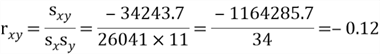
We compute the sample correlation coefficient by this formula:

Where:
![]()
![]()
![]()
![]()
We have already obtained ![]() ,
, ![]() and
and ![]() for the sample data set, shown in Table 8 and 9. Then, we can apply the correlation formula to obtain the value of the correlation coefficient:
for the sample data set, shown in Table 8 and 9. Then, we can apply the correlation formula to obtain the value of the correlation coefficient:
R provides a function, cor( ), to calculate correlation coefficient of variables. We run the following R codes through RTVS.
library(RODBC)
# Load data from data warehouse
dbConnection <-'Driver={SQL Server};Server=.;Database=AdventureWorksDW2017;Trusted_Connection=yes'
channel <- odbcDriverConnect(dbConnection)
InputDataSet <- sqlQuery(channel,
'
        SELECT  [CustomerKey]
              , [YearlyIncome]
              , [Age]
          FROM[dbo].[vTargetMail]
'
)
# Read customer income data to a vector
customer_income <- InputDataSet$YearlyIncome
# Read customer age data to a vector
customer_age <- InputDataSet$Age
# Apply cor function to calculate the covariance
income_age_cor <- cor(customer_income, customer_age)
# Output the correlation for the paried variables
cat("The correlation coefficient:", format(income_age_cor, big.mark =","), "\n")
The correlation coefficient is shown in the R interactive window.
The correlation coefficient: 0.1444071
Table 11 shows the correlation coefficient s of customer yearly income and age for the population data set and the sample data set.
| Population | Sample | |
|---|---|---|
| Correlation | 0.14 | -0.12 |
Table 11 – The Correlation Coefficients of Customer Yearly Income and Age Variables
Professor Jost's rule-of-thumb cutoffs, presented in Table 10, imply that the correlation coefficient of yearly income and age, shown in Table 11, is very weak, which means there is no apparent linear association between these two variables. When a customer age increases, his/her yearly income does not tend to either increase or decrease. This also indicates that there is no conflict between the population correlation coefficient and the sample correlation coefficient. Both calculation results suggest that the pairing of customer yearly income and customer age is purely random.
Summary
Through measures of variability in combination with measures of central tendency, we can obtain a more complete picture of data values in a data set. The first statistic discussed in this tip is range, which is difference between the largest value and the smallest value in a data set. Since range is based on only the two most extreme values, we have introduced the second measure of variability, the interquartile range, which is the range of the middle 50% of the data. Then we have presented three other measures of variability, the average deviation from the mean, the variance and the standard deviation. These three measures are based on measuring distance between every value and the mean in the data set.
Finally, we have used the covariance to find out how two paired variables are related. The covariance is also based on measuring distance from the mean. To describe the degree to which the variables tend to move together, we have used a normalized version of the covariance, i.e. the correlation coefficient.
References
[1] Zhou, N. (2018, November 11). Getting Started with Data Analysis on the Microsoft Platform – Examining Data. Retrieved from https://www.mssqltips.com/sqlservertip/5758/getting-started-with-data-analysis-on-the-microsoft-platform–examining-data/.
[2] Kess, B. (2017, December 12). AdventureWorks sample databases. Retrieved from https://github.com/Microsoft/sql-server-samples/releases/tag/adventureworks/.
[3] Hummelbrunner, S. A., Rak, L. J., Fortura, P., & Taylor, P. (2003). Contemporary Business Statistics with Canadian Applications (3rd Edition). Toronto, ON: Prentice Hall.
[4] William, M., & Sincich, T. (2012). A Second Course in Statistics: Regression Analysis (7th Edition). Boston, MA: Prentice Hall.
[5] Kros, F. J. & Rosenthal A. D. (2015, December). Statistics for Health Care Management and Administration: Working with Excel (3th edition). San Francisco, CA: Jossey-Bass.
[6] Weiers, M. R. (2010, March 17). Introduction to Business Statistics (7th edition). Mason, OH: South-Western College Pub.
[7] Freed, N., Berguist, T. & Jones, S. (2013, November 27). Understanding Business Statistics. Hoboken, NJ: Wiley.
[8] Jost, S. (2017). CSC 423: Data Analysis and Regression. Retrieved from DePaul University Website: http://facweb.cs.depaul.edu/sjost/csc423/
Next Steps
- Descriptive statistics is one major branch of statistics. My other tip [1] has studied measures of central tendency, and this tip has studied measures of variability of data. We can use these two tips to review some fundamental statistics concepts; what is more, we should know how to interpret these measures.
- Check out these related tips:

Nai Biao Zhou has twenty years of experience in software development, with strong analytical skills and a broad range of computer expertise.
He has fifteen years of experience in development and maintenance of database applications on SQL Server in OLTP/OLAP/BI environments.
He has a master’s degree in Control Engineering and is pursuing a Master of Science degree in Predictive Analytics.
Knowledge/Skills
Advanced computer programming skills and well versed with C/C#, Java, ASP.NET, JavaScript, and SQL.
In depth knowledge of Solution Architecture, and Software Development Life Cycle (SDLC).
Microsoft Certified Application Developer (MCAD) since 2004.
- MSSQLTips Awards: Author of the Year – 2021 | Rising Star (50+ tips) – 2024 | Author Contender – 2020, 2023