By: Nai Biao Zhou | Updated: 2021-10-14 | Comments | Related: > TSQL
Problem
Even though there are many new and shiny techniques in the AI/ML area, classic statistical methods such as regression analysis remain powerful and practical (Shin, 2021). The multiple linear regression (MLR) analysis is a statistical procedure that examines the relationship between a response variable and several predictor variables. We then can use an MLR model to make estimations and predictions. Business users may ask IT professionals to build an MLR model and use it for helping to make data-driven decisions at work. However, some IT professionals may have limited knowledge of regression analysis. Therefore, they want to follow a step-by-step procedure to construct a good regression model and apply it in practice.
Solution
Regression analysis uses a mathematical equation to express the relationship between a response variable and a set of predictor variables. It often estimates the magnitude of the impact of one unit of change in one predictor variable on a response variable (Holmes et al., 2017). Data analysts can use statistical tests to assess the usefulness of one or more predictors. In addition, when given a specific data point, they can estimate the mean value of the response variable or predict a single value of the response variable. While data are often specific to various contexts and disciplines, the data analysis approaches tend to be similar (Alexander, 2021). Many companies use regression analysis in the decision-making process to handle all sorts of business issues.
A data analysis project usually starts with problem statements. The problem statements determine what questions the analysis project should address (Chatterjee & Hadi, 2006). Gallo advises that business users narrow the focus when asking data analysts to perform regress analysis (Gallo, 2015). Data analysts may achieve undesired outcomes if they use everything they can get. Furthermore, inaccurate problem statements or the wrong understanding of the problems would result in an erroneous outcome.
This exercise concentrates on a procedure to build a multiple linear regression model. To illustrate the procedure, we study the real estate market in the King Country, the USA. Real estate managers want to investigate what characteristics affect the sales price of a house. They also want to estimate the average price of a group of properties that has the same characteristics. Additionally, they are interested in predicting the sales price for a house that just entered the real estate market. Kaggle hosted a dataset "House Sales in King Country, USA" (Harlfoxem, 2016). In addition, the R package "moderndive" embedded the dataset in the "house_prices" data frame (Ismay & Kim, 2021). For the sake of simplicity, we extract a sample from the data frame "house_price" in this exercise.
We refer to Mendenhall and Sincich’s seven-step procedure (Mendenhall & Sincich, 2012) to build a multiple linear regression model:
- Collect the sample data.
- Hypothesize a form of the model.
- Estimate unknown parameters in the model and select a model.
- Specify the error term distribution and estimate its variance.
- Checking Model Adequacy.
- Statistically evaluate the utility of the model.
- Apply the model in practice.
When walking through the procedure, we use the R language for statistical computing and producing graphics. The R scripts used in this exercise involve these packages: "tidyverse," "moderndive," "gridExtra," "visdat," "Hmisc," "GGally," "reshape2," and "car." All R code works with R 4.0.5 on Windows 10 Pro 10.0 <X64>. To manage and execute R code, the author recommends the integrated development environment (IDE), RStudio.
The author structures the rest of the article as follows. Section 1 explores the data collection and exploratory data analysis (EDA) techniques. Since we have extensive sample data, we split the data into a training dataset and a test dataset. We then hypothesize a form of the model in Section 2. Next, in Section 3, we cover a process to use the ordinary least squares (OLS) method to fit the sample data to a model and estimate the unknown parameters in the model. After obtaining the MLR model equation, we apply an overall F-test to evaluate the model utility. This section also introduces other concepts, such as R-squared, adjusted R-squared, multicollinearity, and influential points. All these have influences on model construction and model selection. We then propose three model selection strategies: backward, forward, and stepwise, and use R code to implement these strategies. Furthermore, to ensure the model be useful in practice, we use the test dataset to validate the model.
Then, Section 4 presents the Gauss-Markov assumptions, a set of seven assumptions. According to the Gauss-Markov theorem, if an MLR model satisfies the first six assumptions, we can obtain the best linear unbiased estimators through the OLS method. Many texts use a set of four model assumptions. The statistical inferences depend on the model satisfying these assumptions. Section 5 uses partial F-tests to answer three types of research questions and evaluate the model utility. Next, we examine the residual plots in Section 6 to check model adequacy. Finally, we apply the model in practice in Section 7. We interpret the impact on the response variable due to the change of the predictor variables, and use the model for estimation and prediction.
1 – Collecting the Sample Data
When using statistics to derive insights from data, we should have data for analysis. Therefore, we must collect data before performing any statistical analysis. We used to select a random sample, a subset of the population, to perform statistical analysis. However, we acknowledge the blurred distinction between a population and a sample with the advent of big data. Nowadays, a company can collect data for an entire population. Nevertheless, sometimes, it is too time-consuming or costly to study the entire population. Therefore, even though the company can obtain data for an entire population, data analysts still prefer to select a random sample.
1.1 Data Collection
Many methods are available for us to collect data. Two of them are well-known: the direct observation method and the experiment method. The critical difference between these two methods is that the direct observation method does not control the predictor variables' values, but the experiment method does. Additionally, when adopting the experiment method, we can increase the amount of information in the data without any additional cost. We may also establish a cause-and-effect relationship among variables when analyzing experimental data. Nevertheless, when we use observational data, a statistically significant relationship between a response and a predictor variable does not necessarily imply a cause-and-effect relationship (Mendenhall & Sincich, 2012). In the business world, it may be impossible to predetermine values for predictor variables; as a result, many regression applications at work use the direct observation method.
In addition to these two popular methods, the use of historical data is also a convenient collection method applied. We can pursue a retrospective study based on historical information (Montgomery et al., 2012). Nowadays, data are business assets and have entered the mainstream in most businesses (Redman, 2008). We apply the knowledge discovery process to detect patterns, gain insight, explain phenomena, and answer concrete business questions. However, we should know that using historical data has some disadvantages. For example, historical data may be less reliable. This exercise uses historical data for regression analysis. We use a data frame embedded in an R package.
1.2 Choice of Relevant Variables
We have defined the problem statements. Then, we can consult subject experts to determine the response variable and a set of predictor variables. The statistical inference depends on the correct choice of variables. We select 19 variables from the "house_prices" data frame:
- price: the sale price of a house in King Country, the USA.
- bedrooms: the number of bedrooms in a house.
- bathrooms: the number of bathrooms in a house.
- sqft_living: square footage of a house.
- sqft_lot: square footage of the lot.
- floors: total floors (levels) in a house.
- waterfront: a house that has a view to a waterfront.
- view: has been viewed.
- condition: how good the condition is overall.
- grade: overall grade given to the housing unit, based on the King County grading system.
- sqft_above: square footage of house apart from the basement.
- sqft_basement: square footage of the basement.
- yr_built: built year.
- yr_renovated: the year when the house was renovated.
- zipcode: zip code.
- lat: latitude coordinate
- long: longitude coordinate
- sqft_living15: the average lot square footage of the 15 closest houses
- sqft_lot15: the average house square footage of the 15 closest houses
The sale price is the response variable, and the other 18 variables are predictor variables. The 18 variables do not explain the variation in response variable equally, and some are more significant than others. Professor Jost gave good advice in obtaining a good regression model. He pointed out, "A good regression model must be accurate (have a higher adjusted R-squared), but it must also be parsimonious (as few predictor variables as possible). In addition, its residuals must be well behaved (unbiased, homoscedastic, independent, and normal)" (Jost, 2017). We follow the seven-step procedure to find the acceptable model to answer the questions in the problem statements.
1.3 Data Preparation
Without loss of generality, we select a sample from the "house_prices" data frame. When introducing observational data, Mendenhall and Sincich recommend that the sample size be greater or equal to 10 times the number of unknown parameters in a multiple linear regression model (Mendenhall & Sincich, 2012). We adopt their guidelines. Thus, the sample size should be at least 190. Furthermore, when selecting a large sample size, e.g., >3000, we can use linear regression techniques even though the response variable does not have a normal distribution (Li et al., 2012).
The "house_prices" data frame has 21,613 rows; therefore, we can select a large sample from this dataset. We want to use a training dataset to find the model and a test dataset to validate the model. We selected 6004 rows and split them into a training set and a test set. Numerous approaches can achieve data partitioning. We use a straightforward one in this exercise. The following R code generates the sample set, the training set, and the test set:
# The core tidyverse includes the packages that we use in everyday data analyses.
# https://www.tidyverse.org/
library(tidyverse)
# The package contains the house_prices data frame
library(moderndive)
#1. Load the housing data frame and assign it to a variable
house.prices <- data.frame(house_prices)
#2. Set the seed so that the sample can be reproduced
set.seed(314)
#3. Select random rows from a data frame
house.prices.sample <- sample_n(house.prices, 6004)
#4. Split the sample into training and test datasets
set.seed(314)
#5. Select 50% of integers from 1 to nrow(house.prices) randomly
random.row.number <- sample(1:nrow(house.prices.sample),
                            size=round(0.5*nrow(house.prices.sample)),
                            replace=FALSE)
#6. Takes rows that are in random integers
training.set <- house.prices.sample[random.row.number,]
#7. Takes rows that are NOT in random integers
test.set <- house.prices.sample[-random.row.number,]
#-------------------------------------------------------------------------------
# The following sections access the data frames house.prices.sample directly
#-------------------------------------------------------------------------------
1.4 Exploratory Data Analysis
In an ideal world, according to the problem statements, we collect corresponding data. However, we often analyze data collected for other purposes (Johnson & Myatt, 2014). Therefore, a critical step in a data analysis project is to understand the data. Exploratory data analysis (EDA) techniques help perform initial investigations on data. We can discover patterns, spot anomalies, test hypotheses, and check assumptions (Patil, 2018). EDA techniques, initially developed by American mathematician John Tukey in the 1970s, help understand variables and relationships among them; we then choose appropriate statistical techniques for data analysis (IBM Cloud Education, 2020). Mazza-Anthony provides a framework for us to perform an effective EDA (Mazza-Anthony, 2021).
1.4.1 Check for Missing Data
Data collected in the real world may not be complete. The cause of missing values might be data corruption or failure to record data. There are three types of missing data: Missing Completely at Random (MCAR), Missing at Random (MAR), and Missing Not at Random (MNAR) (Banjar et al, 2017). When MCAR occurs, missing data is not related to other variables. Therefore, the data is unbiased. However, data are rarely MCAR. Next, MAR does not depend on things not observed. The third type, MNAR, the worst case, depends on both observed and unobserved factors. Categorizing missing data into these types help us to handle the remaining data correctly.
Many data science algorithms, generally, do not work well in the presence of missing data (Kumar, 2020). We are not fully confident in the analysis output derived from a dataset with missing values. Therefore, when performing EDA, we start with missing data analysis (MDA). We then determine techniques to handle these missing values. Both Kumar (Kumar, 2020) and Swalin (Swalin, 2018) wrote excellent articles to introduce missing data handling. Han and his co-authors concluded six methods to fill the missing values (Han et al., 2012):
- Ignore the missing values.
- Fill in the missing value manually.
- Use a global constant to fill in the missing value.
- Use a measure of central tendency for the attribute (e.g., the mean or median) to fill in the missing value.
- Use the attribute mean or median for all samples belonging to the same class as the given tuple.
- Use the most probable value to fill in the missing value.
The R package "visdat" provides functions to glance at the data. The package provides tools, including the functions "vis_dat()" and "vis_miss()," to create heatmap-like visualization. First, we use the "glimpse()" function to get a peek at the sample and get familiar with the columns and their corresponding data types:
 glimpse(house.prices.sample)
# Output of the glimpse function:
# > glimpse(house.prices.sample)
# Rows: 6,004
# Columns: 21
#   $ id            <chr> "7936500190", "8712100530", "5466380050", ~
#   $ date          <date> 2014-10-21, 2014-08-13, 2014-12-19, 2014-~
#   $ price         <dbl> 1339000, 895000, 304500, 240000, 1800000, ~
#   $ bedrooms      <int> 4, 4, 4, 2, 4, 3, 3, 4, 3, 4, 4, 2, 6, 5, ~
#   $ bathrooms     <dbl> 3.75, 2.00, 2.50, 1.00, 3.50, 2.50, 1.00, ~
#   $ sqft_living   <int> 2130, 1710, 2030, 670, 4460, 2196, 1590, 2~
#   $ sqft_lot      <int> 34689, 4178, 5202, 10920, 16953, 7475, 540~
#   $ floors        <dbl> 1.5, 1.5, 2.0, 1.0, 1.0, 2.0, 1.0, 2.0, 1.~
#   $ waterfront    <lgl> TRUE, FALSE, FALSE, FALSE, FALSE, FALSE, F~
#   $ view          <int> 4, 0, 0, 0, 0, 0, 1, 0, 0, 0, 0, 0, 0, 0, ~
#   $ condition     <fct> 3, 4, 3, 3, 3, 3, 3, 4, 3, 4, 3, 3, 4, 3, ~
#   $ grade         <fct> 9, 8, 8, 6, 9, 8, 8, 8, 8, 7, 8, 7, 7, 8, ~
#   $ sqft_above    <int> 2130, 1710, 2030, 670, 2550, 2196, 1280, 2~
#   $ sqft_basement <int> 0, 0, 0, 0, 1910, 0, 310, 0, 0, 500, 0, 0,~
#   $ yr_built      <int> 1955, 1926, 2001, 1942, 1962, 2006, 1948, ~
#   $ yr_renovated  <int> 0, 0, 0, 0, 1994, 0, 0, 1987, 0, 0, 0, 0, ~
#   $ zipcode       <fct> 98136, 98112, 98031, 98146, 98039, 98030, ~
#   $ lat           <dbl> 47.5489, 47.6373, 47.3880, 47.5128, 47.633~
#   $ long          <dbl> -122.398, -122.300, -122.176, -122.372, -1~
#   $ sqft_living15 <int> 3030, 1760, 2260, 900, 1980, 1860, 2140, 2~
#   $ sqft_lot15    <int> 28598, 4178, 5232, 7425, 13370, 6755, 7161~
#   >
We then use the "vis_dat()" and "vis_miss()" functions to visualize the data class structure and missingness. Because the initial dataset is large, we analyze the sample data to avoid a possible computer memory issue. We also only look at the columns of interests. The following R code invokes these two functions to produce two plots, respectively. Figure 1 indicates that the dataset has factors, integers, logical and numeric values, without any missing values. Figure 2 shows the percentage of missingness in the dataset. Fortunately, the dataset does not have any missing value. Tierney’s article (Tierney, 2019) demonstrates a custom plot when discovering missing data in a dataset.
# https://cran.r-project.org/web/packages/visdat/vignettes/using_visdat.html
library(visdat)
# Removing uninterested columns with dplyr
house.prices.sample   %>%
  select(-c(id,date)) %>%
# Explore the data class structure and missingness
vis_dat(sort_type = FALSE) +
  ggtitle("Explore the Data Class Structure and Missingness") +
  theme(plot.title = element_text(hjust = 0.5,size=20))
house.prices.sample   %>%
  select(-c(id,date)) %>%
# A custom plot for missing data.
vis_miss(sort_miss = TRUE, cluster = TRUE) +
  ggtitle("The Percentages of Clustered Missingness ") +
  theme(plot.title = element_text(hjust = 0.5,size=20)
        ,axis.text.x = element_text(angle = 90))
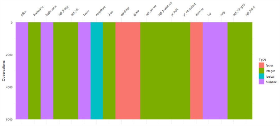
Figure 1 Explore the Data Class Structure and Missingness
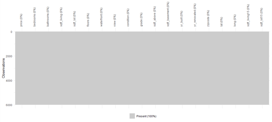
Figure 2 The Percentage of Clustered Missingness
1.4.2 Obtain Summary Statistics
When checking for missing data, we already know that the sample set has factors, integers, logical and numeric values. The factor, a data structure in R programming, represents a pre-defined, finite number of values. Therefore, a factor column in R describes a categorical variable storing both string and integer data values as levels. A categorical variable could be either a nominal or an ordinal (Zhou, 2019). After reviewing the three factors in the sample, we find these features are ordinal categorical variables. For simplicity, we assume they are equally spaced. Then, it is reasonable to treat these ordinal categorical variables as continuous (i.e., numeric) variables (Pasta, 2009). We can also consider the logical variable to be a numeric variable with values 0 and 1.
Summary statistics summarize information about sample data. We can use R functions to obtain summary statistics. For example, the "summary()" function gives us the basic statistics of a dataset like minimum, first quartile, mean, median, third quartile, and maximum (Soetewey, 2020). We use the following R code to transform the sample data and provide summary information.
house.prices.sample %>%
  select(-c(id, date))                        %>%
  mutate(condition = as.numeric(condition))   %>%
  mutate(grade = as.numeric(grade))           %>%
  mutate(zipcode = as.numeric(zipcode))       %>%
  mutate(waterfront = as.numeric(waterfront)) %>%
  summary()
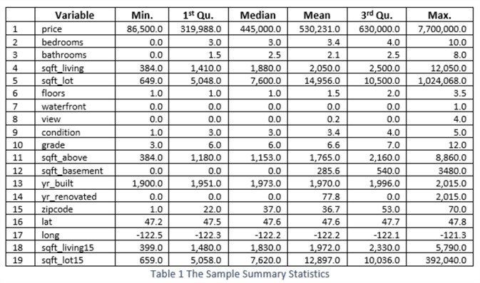
We reorganize the output into Table 1 for easy reading. We observe that the variables "price," "sqft_lot," and "sqft_lot15" vary by several orders of magnitude. The value of the "yr_renovate" suddenly increases. Ideally, we do not expect a significant gap in data points. When two or more variables have even distributions across the ranges, it is easy to detect their relationship; moreover, we can produce a good visualization. When determining to the application of data transformation techniques, we need to take these findings into account.
1.4.3 Identify the Shape of the Data
We often use a histogram to plot frequency distributions of a numeric variable (Yi, 2019). At first glance, the histogram looks like a bar chart because both have a series of bars. However, there are essential differences between them. For example, a histogram presents numerical data, whereas a bar graph shows categorical data. After type conversion, the sample data we selected includes 19 numerical variables; therefore, we use histograms to examine their frequency distributions.
We can use ggplot2 to plot a histogram with an excellent appearance and feeling. However, as observers of these charts, we want to look at the shape of the data quickly and can use the "hist.data.frame" function, which draws a matrix of histograms. The matrix allows us to examine the shape of each variable’s distribution immediately.
# Contains many functions useful for data analysis, high-level graphics
library(Hmisc)

house.prices.sample %>%
  select(-c(id, date))                        %>%
  mutate(condition = as.numeric(condition))   %>%
  mutate(grade = as.numeric(grade))           %>%
  mutate(zipcode = as.numeric(zipcode))       %>%
  mutate(waterfront = as.numeric(waterfront)) %>%
  # Plot the histogram matrix
  hist.data.frame()
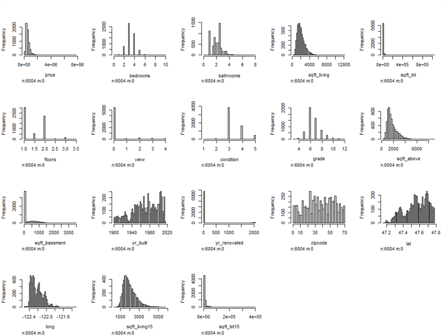
Figure 3 Histograms for Variables in the Sample
The summary statistics told us three variables, "price," "sqft_lot," and "sqft_lot15," are different from others. Figure 3 demonstrates that most values of these three variables are on the left side of the histograms, which means most have low values. The histograms also show that a significant number of houses do not have a basement, and many houses are non-renovated. Some variables, for example, "sqft_living," "sqft_above," and "sqft_living15," have approximately normal distributions with skewness. Other variables, such as "bathroom," "yr_built," "lat," and "long," have multimodal distributions.
However, The function "hist.data.frame()" does not plot a histogram for the variable "waterfront," which is a numeric variable containing values of 0 and 1. Since the variable can only take a small set of values, we can use a bar chart to examine the distribution (Wickham & Grolemund,2017). We use the following code to plot the bar chart, shown in Figure 4. We observe that the percentage of a house having a view to a waterfront is very low.
house.prices.sample %>%
  select(-c(id, date))                        %>%
  mutate(condition = as.numeric(condition))   %>%
  mutate(grade = as.numeric(grade))           %>%
  mutate(zipcode = as.numeric(zipcode))       %>%
  mutate(waterfront = as.numeric(waterfront)) %>%
  # Plot the bar chart
  ggplot(aes(waterfront)) +
  geom_bar(width = 0.1) +
  xlab("Waterfront") +
  ylab("Count") +
  ggtitle("Number of Houses which have a View to a Waterfront") +
  theme_bw()  +
  theme(plot.title = element_text(hjust = 0.5,size=16),
        axis.title = element_text(size=12))
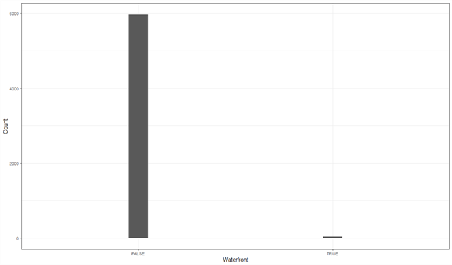
Figure 4 Number of Houses which have a View to a Waterfront
1.4.4 Describe Significant Correlations
When building a simple linear regression model, we use a scatter plot to visualize and examine the relationship between the response and predictor variables (Zhou, 2020). Suppose the visual aid does not suggest there is, at least, somewhat of a linear relationship. In that case, we may apply other techniques, for example, data transformations. Multiple linear regression is an extension of simple linear regression. Many ideas we use in simple linear regression can carry over to the multiple regression setting (Kiernan, 2014). Therefore, we should study the relationships between the response variable and each predictor variable as well. Additionally, we should also check the relationships between predictor variables. Multicollinearity, which is undesirable, occurs when at least one predictor variable highly correlates with another predictor variable.
Rather than creating a scatter plot for each pair of variables, individually, we can create a correlation matrix that illustrates the linear correlation between each pair. R provides several functions to produce a correlation matrix. In this exercise, we use the function "ggpairs()" from the GGally package (Finnstats, 2021). The correlation matrix helps check linearity between the response variable and predictor variables. We can also detect collinearity among the predictor variables. We use the following R code to produce the correlation matrix, shown in Figure 5. It is worth noting that the execution time of these scripts takes longer than other scripts.
# https://r-charts.com/correlation/ggpairs/
library(GGally)

house.prices.sample %>%
  select(-c(id, date))                        %>%
  mutate(condition = as.numeric(condition))   %>%
  mutate(grade = as.numeric(grade))           %>%
  mutate(zipcode = as.numeric(zipcode))       %>%
  mutate(waterfront = as.numeric(waterfront)) %>%
  # Plot the Scatter Plot Matrix
  ggpairs() +
  ggtitle('The Scatter Plot Matrix') +
  theme_bw()  +
  theme(plot.title = element_text(hjust = 0.5,size=20))
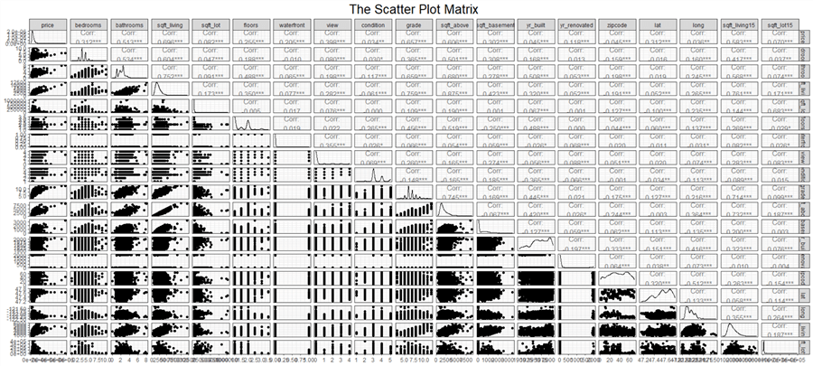
Figure 5 The Scatter Plot Matrix
The upper triangle in the scatter plot matrix shows the linear correlation coefficients, suggesting the linear dependence level between every two variables. The lower diagrams are the scatter plots, which visualize the relationship between each pair of two variables. The interpretation of correlation coefficients varies from research area to research area. There is no absolute rule to interpret the strength of the correlation. We select a conventional approach to interpret a correlation coefficient (Schober et al., 2018).
The first row indicates that the response variable has strong positive linear relationships (r>=0.7) with the predictor variable "sqft_living." The response variable has moderate positive linear relationships (0.4<=r<=0.69) with predictor variables "bathrooms, "grade," "sqft_above," and "sqft_living15." However, the response variable has negligible correlations (0<=r<=0.1) with "sqft_lot," "condition," "yr_built," "zipcode," "long," and "sqft_lot15." The rest of predictor variables have weak correlations (0.1<=r<=0.39) with the response variable.
Moreover, we observe that collinearity occurs. For example, the predictor variables "sql_living" and "sql_above" have a strong positive linear relationship (r = 0.875), which is significant (p < 0.001). Note that the symbol "***" implies the p-value is less than 0.001. However, multicollinearity is hard to detect since it might not be visible on the scatter plot matrix.
1.4.5 Spot Outliers in the Dataset
We call an observation an outlier when the observation lies an abnormal distance from other values in a sample (Birkett, 2019). Many reasons might make an outlier occur, for example, a measurement or recording error. In addition, outliers may be either valuable or meaningless. Therefore, it is crucial to detect outliers in a dataset. We can graph data to identity outliers (Renjini, 2020). The boxplot, histogram, and scatterplot are visualization techniques for identifying outliers. When we use a boxplot to identify outliers, an outlier is a data point located outside the boxplot's whiskers (Dong, 2012). The following R code is used to plot boxplots for five selected variables for demonstration purposes. Of course, we should examine all variables when working on an actual project.
# https://towardsdatascience.com/reshape-r-dataframes-wide-to-long-with-melt-tutorial-and-visualization-ddf130cd9299
library(reshape2)

house.prices.sample           %>%
  select(c(bedrooms,bathrooms,floors, condition,grade))  %>%
  sample_n(6004)                              %>%
  mutate(condition = as.numeric(condition))   %>%
  mutate(grade = as.numeric(grade))           %>%
  mutate(id = row_number())                   %>%
  melt(id=c('id'))                            %>%
  # The boxplot
  ggplot(aes(x=variable, y=value)) +
  geom_boxplot() +
  xlab("The Selected Variables") +
  ylab("Values") +
  ggtitle("The Boxplot for Five Selected Variables") +
  theme_bw()  +
  theme(plot.title = element_text(hjust = 0.5,size=20),
        axis.title = element_text(size=16))
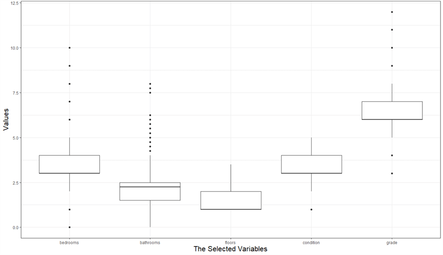
Figure 6 The Boxplot for Five Selecetd Variables
We observe a small number of outliers in Figure 6. These values are extreme values that deviate from others in the sample. They probably are not data errors; therefore, we cannot simply remove them. However, these outliers may affect performing statistical analysis, probably leading to problems. Garrett provides four approaches to deal with outliers (Garrett, 2020). There are also other strategies for dealing with outliers in data (Birkett, 2019). We should choose appropriate approaches according to analysis objectives, business context, intended outcome, and datasets.
1.5 Data Transformation
Data transformations, an essential and popular tool in data analysis for addressing various practical issues, use mathematical approaches to modify values of a variable; some commonly discussed data transformation techniques are square root, log, and inverse (Osborne, 2002). Other techniques include adding constants, normalization, and discretization. However, Dr. Osborne warned that data transformation fundamentally changes the variables' nature, making the interpretation more complex. Thus, we should use data transformations with care.
A data analysis project employs data transformations, more or less. We always use data transformations to correct some known issues within data. The primary use of data transformations is to help the interpretation. We usually develop data transformations for these four purposes:
(1), Enhance the interpretation of the impact of predictor variables on the response variable.
(2), Resolve the issue of contamination by outliers in sample data.
(3), Address non-normality of errors in linear regression.
(4), Express non-linear relationships between a response variable and predictor variables to linear ones; in fact, a linearizing transformation ideally would simultaneously normalize the residuals (Pek et al., 2017).
We find a big gap in the "yr_renovated" data when looking at the scatter plot matrix. When examining the values, we find they have different meanings, i.e., attribute overloading. For example, the value of zero means non-renovated. However, the non-zero value means the year when the house renovation occurred. Therefore, the fact that the variable changes from 0 to 1934 does not mean an increase of 1934 units. To fix this data quality issue, we can classify houses into two categories: renovated and non-renovated. We then can examine the difference between a renovated house and a non-renovated house. Therefore, we create a new variable, denoted by "bln_renovated." The new variable substitutes the old variable and takes values 0 and 1:

When observing any curvilinear relationship in the scatter plot matrix, we may want to linearize it. Usually, the first step is to transform predictor variables. If the transformation does not achieve a linear relationship, we attempt to transform the response variables. Choosing a correct transformation technique is a process of trial and error. Since data transformations change the nature of data, we should apply transformation techniques only to correct issues within the data. For example, the response variable "price" in the dataset varies in several orders of magnitude, but most others do not. Therefore, we apply log transformation to the variable to detect linear relationships. We also apply log transformation to "sqft_lot," and "sqft_lot15."
When using the least-squares method to compute unknown parameters of a linear regression equation, we do not assume the normality of any variable. Therefore, it is not always necessary to transform data for normality. However, we assume that the error component has a normal distribution when drawing the statistical inference, such as in constructing confidence intervals and conducting t-tests. We can evaluate this assumption by examining the normality of the residuals. Bear in mind that we should transform data for particular reasons.
Nevertheless, when the sample size is large (e.g., > 25 for each group in a t-test), the assumption of normality can be relaxed. These unknown parameters are approximately normally distributed around the true parameter values in a large sample due to the central limit theorem (Pek et al., 2017). In this exercise, we selected 3002 rows to train the model. Therefore, even though the response variable violates the "normality assumption" rule, using the linear regression technique remains valid (Li et al., 2012).
We use the following code to implement the data transformation. The subsequent
steps use the transformed data. It is good to plot the scatter plot matrix again
and look at the improvement due to data transformation.
Figure 7
illustrates the new matrix. The transformation has not improved the linearity significantly,
but the transformed response variable has an approximately normal distribution.
In addition, the scatter plots in the first column indicate fewer outliers in the
response variable. For the transformed response variable,
 ,
one unit increase in
 is equivalent to an increase of 900% in the original scale of the response variable.
# The core tidyverse includes the packages that we use in everyday data analyses.
# https://www.tidyverse.org/
library(tidyverse)
# The package contains the house_prices data frame
library(moderndive)
#1. Load the housing data frame and assign it to a variable
house.prices <- data.frame(house_prices)
#2. Set the seed so that the sample can be reproduced
set.seed(314)
#3. Select random rows and transform data
house.prices.sample.transform <- sample_n(house.prices, 6004) %>%
  mutate(condition = as.numeric(condition))   %>%
  mutate(grade = as.numeric(grade))           %>%
  mutate(zipcode = as.numeric(zipcode))       %>%
  mutate(waterfront = as.numeric(waterfront)) %>%
  mutate(price_log = log10(price))            %>%
  mutate(sqft_lot_log = log10(sqft_lot))      %>%
  mutate(sqft_lot15_log = log10(sqft_lot15))  %>%
  mutate(bln_renovated =case_when(
    yr_renovated == 0 ~ 0,
    TRUE ~ 1))                                %>%
  select(c("price_log","bedrooms","bathrooms","sqft_living",
           "sqft_lot_log","floors","waterfront","view",
           "condition","grade","sqft_above","sqft_basement",
           "yr_built","bln_renovated","zipcode", "lat",
           "long","sqft_living15","sqft_lot15_log"))
#4. Split the sample into training and test datasets
set.seed(314)
#5. Select 50% of integers from 1 to nrow(house.prices) randomly
random.row.number <- sample(1:nrow(house.prices.sample.transform),
                            size=round(0.5*nrow(house.prices.sample.transform)),
                            replace=FALSE)
#6. Takes rows that are in random integers
training.set.transform <- house.prices.sample.transform[random.row.number,]
#7. Takes rows that are NOT in random integers
test.set.transform <- house.prices.sample.transform[-random.row.number,]
#-------------------------------------------------------------------------------
# The following sections access the data frames, house.prices.sample.transform,
# training.set.transform and test.set.transform directly
#-------------------------------------------------------------------------------
# https://r-charts.com/correlation/ggpairs/
library(GGally)
# Plot the Scatter Plot Matrix
ggpairs(house.prices.sample.transform) +
  ggtitle('The Scatter Plot Matrix') +
  theme_bw()  +
  theme(plot.title = element_text(hjust = 0.5,size=20))
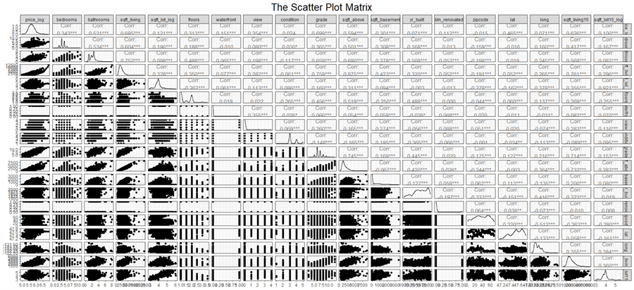
Figure 7 the Scatter Plot Matrix Produced from Transformed Data
2 – Hypothesizing a Form of the Model
The term "model" represents any phenomenon by using a mathematical framework. For example, a regression model demonstrates the functional relationship among variables. We can think that models exist in nature but are unknown (Shalabh, 2020). In regression analysis, researchers hypothesize a form of the model and then compute the estimator of the unknown parameters. Sometimes, prior knowledge can give us some hints about the form. The selected form determines the success of the regression analysis. When the researchers find that the regression model is not useful in the adequacy checking and validation phase, they use another hypothesized form. Thus, regression analysis is an iterative procedure.
We often see one response variable in regression modes; however, the response variable could be a set of variables. When a regression model has one response variable, the model is a univariate regression model. On the other hand, a multivariate regression model has two or more response variables (Chatterjee & Hadi). The number of predictor variables determines if a regression is a simple regression or a multiple regression. Therefore, we should not confuse simple regression with univariate regression and multiple regression with multivariate regressions. This article considers only univariate regression; therefore, the term regression means univariate regression in the context.
2.1 General form of a Regression Model
Regression models have four components (Wikipedia, 2021):
- The unknown parameters
 .
.
- The predictor variables
 .
.
- The response variable
 .
.
- The error component

We represent a regression model with the following mathematic equation:

The function
 usually has a constant term,
 .
The constant term may be meaningless, but a regression model should generally include
a constant (Frost, 2018). The other unknown parameters determine the contribution
of the predictor variables. The error component reflects the stochastic nature of
the model. When
 ,
the equation represents a mathematical model otherwise a statistical model (Shalabh,
2021)
By definition, a model is said to be linear when it is linear in parameters. Formally speaking, when we say a regression model is linear, all the partial derivatives of the response variable y with respect to any of the parameters are independent of the parameters. On the contrary, the regression model is non-linear if some partial derivatives are not independent of the parameters. When a response variable has linear relationships with predictor variables, the model may not be linear. For example, the following mathematic equations represent a linear model and non-linear model, respectively (Shalabh, 2020):
- Linear Model:

- Non-linear Model:

In the linear model, we observed that
 ,
,
 ,
and
,
and
 are functions of predictor variables, respectively. These functions are square,
square root, and logarithmic. The term "linear" does not describe the
relationship between the response variable and predictor variables. However, it
indicates that the parameters enter the equation linearly. Thus, compared to non-linear
regression, linear regression is easier to use and more straightforward to interpret.
In addition, R-squared is not valid for non-linear regression, and we cannot calculate
p-values when estimating parameters. Therefore, a general regression guideline suggests
using a linear regression model to represent a phenomenon (Frost, 2018).
2.2 General form of a Multiple Linear Regression Model
The business problems in this exercise want to investigate the relationships
between the sale price of a house in King Country, the USA, and house characteristics.
Thus, the response variable is the price (the sale price of a house). The predictor
variables represent characteristics, such as bedrooms (the number of bedrooms in
a house), sqft_living(the square footage of the house), and sqft_basement ( the
square footage of the basement). Let
 denote the response variable and
 denote predictor variables respectively.
 denote unknown regression parameters respectively, and
 denote error component. We then can write the multiple linear regression in this
form (Mendenhall & Sincich, 2012):

It is convenient to write a multiple regression model in a matrix form for all n data points simultaneously:

where
 is the response vector,
 is the design matrix,
 is the vector of parameters, and
 is the error vector:

3 – Estimating Unknown Parameters in the Model
In practice, we cannot measure X and y in the entire population; therefore, the
true value of
 is unknown. However, we can use sample data to estimate the unknown vector
 .
We use
 to denote the estimator, and the "hat" means "estimator of."
Thus, given any data point, e.g.,
 we can obtain the estimator of
 :
:

or

We also call this equation the estimated multiple regression equation. The difference
between the
 and its estimator
 measures how well the regression equation fits an individual data point. We call
the difference residual, use
 to denote the residual:

Unlike
 ,
which is unknown,
 is known, and we can compute the vector of residual
 :
:

This exercise uses the method of ordinary least squares (OLS) to find the estimators. To make the estimators reflect the actual parameters, we have four OLS assumptions (Hanck et al., 2020):
- The response variable at any data point has an independent and identical distribution (i.i.d.).
- The residuals must not exhibit any systematic pattern.
- Large outliers are unlikely.
- No perfect multicollinearity.
3.1 Ordinary Least Squares
The method of OLS is a standard approach in regression analysis. We use this method to approximate the solution of over-determined systems of linear equations. An over-determined system has more equations than unknown parameters. Least squares mean that the solution minimizes the sum of the squares of the residuals made in solving every single equation. First, we calculate the sum of squares for residuals (SSE) through this definition:

We arrange the residuals in an
 vector and use
 to denote it. We then rewrite the SSE definition:

We know these facts:
- The vector
 is an
is an
 vector of observations on the response variable; therefore
 is an
is an
 vector.
 - The matrix
 is an
is an
 matrix of observations on
 predictor variables for
 observations.
 is an
is an
 matrix.
 - The vector
 is an
is an
 vector of coefficient estimators, and
 is an
is an
 vector.
 -

Therefore, we can draw these conclusions:
 is transpose of
 ,
and both are a scalar. Since the transpose of a scalar is still the same scalar,
we obtain this equation:

Then, we write the SSE definition:

Let
 be a constant,
 ,
and
,
and
 be
be
 vectors, and
 be a symmetric matrix. Suppose that
 and
and
 are independent, while they are a function of
 .
In addition,
 is independent of
 .
Here are some propositions about matrix differentiation:


Review the SSE equation we just derived. To find a vector
 that minimizes SSE, we can take the derivative of the equation with respect to
 and set the vector partial derivative to the zero vector:

The OLS assumptions state that each
 in the
 vector is independent, and all of them have identical distributions. By using the
matrix differentiation that we just reviewed, we obtained the following equation:

We arrange the equation to obtain the normal equation:

Then solve
 to obtain this formula:

The formula helps explain another OLS assumption: no perfect multicollinearity
(Espinoza, 2012). When
 is column-rank deficient, i.e., one or more columns is equal to a linear combination
of others, the matrix
 is not invertible. We call this problem multicollinearity. It seems we have p predictor
variables, but some of them are linear combinations of others. When several predictor
variables appear to be in a linear relationship, but not precisely, the matrix
 is significantly large and the estimated coefficients are not meaningful.
When multicollinearity occurs, some predictor variables do not contribute information
to the model. A simple way to deal with multicollinearity is to remove these predictor
variables. We can examine the scatter plot matrix to detect linear relationships
between pairs of predictor variables. A multicollinear relationship involving more
than two variables might be invisible on a pair plot. Section
3.5
discusses multicollinear in more depth. After eliminating the predictor variable
"sqft_living,"
we can compute
 using R. We then use the following R code to calculate the estimated coefficients
according to the training dataset.
#1. Create the first column of X
intercept.vector <-  replicate(nrow(training.set.transform), 1)
#2. Construct The predictor variables matrix
training.set.matrix <- training.set.transform       %>%
  select(-c(price_log,sqft_living))                 %>%
  data.matrix()
#3. Construct the X matrix
X <- cbind(intercept = intercept.vector, training.set.matrix)
# Construct the vector y
y <- training.set.transform             %>%
  select(c(price_log))                  %>%
  data.matrix()
#4. Compute the estimator of beta
beta.hat <- solve(t(X)%*%X)%*%t(X)%*%y
beta.hat
#5. Print the estimator of beta
# intercept      -2.521458e+01
# bedrooms       -5.500492e-03
# bathrooms       2.029720e-02
# sqft_lot_log    3.005101e-02
# floors          3.712910e-02
# waterfront      1.414066e-01
# view            3.082094e-02
# condition       2.123608e-02
# grade           6.275603e-02
# sqft_above      6.239232e-05
# sqft_basement   6.552893e-05
# yr_built       -1.592935e-03
# bln_renovated   4.504376e-02
# zipcode        -7.608754e-04
# lat             6.070744e-01
# long           -3.626599e-02
# sqft_living15   5.579294e-05
# sqft_lot15_log -5.064636e-02
The other relevant sums of squares in multiple linear regression models are sum of squares total (SST) and sum of squares for regression (SSR):


For multiple regression models, we have this remarkable property:

3.2 Some Properties of the OLS Method for Multiple Linear Regression
Since we already know
 ,
we can rewrite the equation to obtain this equation:
 .
Substituting
 in the normal equation, we find a very important property of the OLS method:


Then, we have this property of the OLS method for multiple linear regression:

We write the property in a matrix form:
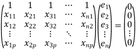
We now can derive some other properties:
1, Each column in
 ,
for example, the jth column
 is uncorrelated with the residual.

Especially, when we look at the first column in the
 ,
we obtain this equation:

Since the first column is a column of ones, we have this property:

This equation indicates that the sum of the residuals is zero; and the sample mean of the residual is zero as well. Let us write the equation in summation notation:

However, to ensure the OLS method performs well, we assumed the residuals should have a zero conditional mean (Hanck et al., 2020). This assumption indicates that the residuals should not show any pattern.
2, The estimator
 is uncorrelated with the residual:

Now, we can prove the equation
 :
:
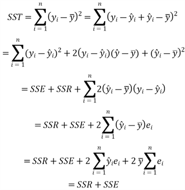
Suppose that
 is the number of observations, and
 is the number of predictor variables. The degrees of freedom for SST are
 ,
the degrees of freedom for SSR are
 and the degrees of freedom for SSE are
 .
We then define the following terms for analysis of variance (ANOVA) F-Test:
- Mean Squares Total:

- Mean Squares Regression:

- Mean Squares Error:

- Standard Deviation of the Residuals:

In general, we want the variation due to the regression to be larger than the variation due to the residuals.
3.3 Overall F-test
Section 3.1 computed the estimated regression coefficients using a sample; however, the true regression coefficients for the population model are unknown. We might obtain these estimated coefficients by chance, and the true values are all zeros. In other words, the response variable may not depend on any predictor variables. If so, we cannot use these predictor variables to make any prediction, i.e., the model is not adequate for predicting. To determine whether the regression model contains at least one predictor variable that is useful in predicting, we can conduct a test of the unity of the model. Here are the null hypothesis and alternative hypothesis:

The test statistic is an F statistic (Mendenhall & Sincich, 2012); and we can compute the test statistic using the following equation:

The test statistic measures the fraction of the variability in the response variable that the model explains. When the test statistic is greater than an F critical value, we can reject the null hypothesis. In that case, we find sufficient evidence against the null hypotheses, which the response variable has no linear relationship with any predictor variable. An F-table or statistical tool can provide the F critical value. The test statistic is not the only measure of significance used in an F Test. In practice, we usually consider the p-value.
Dr. Jost summarized a five-step process to conduct the overall F-test for regression (Jost, 2017):
- State the null and alternative hypotheses.
- Compute the test statistic
- Find the F critical value
- Accept the null hypothesis if the test statistic is less than the F critical value; reject otherwise.
- Use statistical software to determine the p-value.
We use the following R code to implement the five-step process. The value of the F-statistic, which is 559.7, agrees with the value in the model summary. Since the F-statistic is greater than the F critical value, we reject the null hypothesis in favor of the alternative hypothesis. The data provide sufficient evidence that at least one of the model coefficients is non-zero. Many statistical tools, like R, compute the p-value of a statistical test. If the null hypothesis is true, the p-value is the probability of obtaining a test statistic value as extreme or more than that calculated from the sample. Most researchers compare the selected α value to the p-value to make the decision. Since p-value: < 2.2e-16, we reject the null hypothesis. The overall model appears to be statistically useful for predicting house prices.
# Problem Statement:  For a multiple regression model with n = 3002 observations
# and p = 17 predictor variables, test the null hypothesis that all of the
# regression parameters are zero at the 0.05 level.
n <- 3002
p <-17
# 1, State the null and alternative hypothesis
#      H0: Beta.1 = Beta.2 = Beta.3, ... ,= Beta.p
#      H1: Beta.i != 0 for some i
# 2, Compute the test statistic
# 2.1 Fit a Regression Model with all predictor variables
full.model <- lm(price_log~bedrooms+bathrooms+sqft_lot_log+floors+
                   waterfront+view+condition+grade+
                   sqft_above+sqft_basement+yr_built+bln_renovated+
                   zipcode+lat+long+sqft_living15+
                   sqft_lot15_log, data=training.set.transform)
# 2.2 Calculate SSE, SSR, SST, MSE, MSR and MST
# 2.2.1 Compute SSE, MSE
SSE <- sum((training.set.transform$price_log - fitted(full.model))^2)
# The number of df associated with SSE is n–(p+1) because
# p+1 df are lost in estimating the p+1 coefficients.
MSE <- SSE/(n-p-1)
print(paste("SSE:",formatC(SSE, format = "e", digits = 3),
            "MSE:",formatC(MSE, format = "e", digits = 3)))
# 2.2.2 Compute SSR, MSR
SSR <- sum((fitted(full.model) - mean(training.set.transform$price_log))^2)
MSR = SSR/p
print(paste("SSR:",formatC(SSE, format = "e", digits = 3),
            "MSR:",formatC(MSE, format = "e", digits = 3)))
# 2.2.3 Compute SST, MST
SST <- SSR + SSE
MST = SST/(n-1)
print(paste("SST:",formatC(SST, format = "e", digits = 3),
            "MST:",formatC(MSE, format = "e", digits = 3)))
# 2.3 Compute F-Static
F.static <- MSR/MSE
print(paste("F static:", F.static))
# 3 Find a (1 - α)100% F critical value for (p, n-p-1) degrees of freedom
F.critical.Value <- qf(.95, df1=p, df2=n-p-1)
print(paste("The 95th percentile of the F distribution",
            "with (16, 2958) degrees of freedom is:", F.critical.Value))
# 4 Accept the null hypothesis if F.static < F.critical.value; reject it otherwise.
# 5 Use statistical software to determine the p-value.
summary(full.model)
#Printout
#Residual standard error: 0.1103 on 2984 degrees of freedom
#Multiple R-squared:  0.7613,Adjusted R-squared:  0.7599
#F-statistic: 559.7 on 17 and 2984 DF,  p-value: < 2.2e-16
3.4 R-squared and Adjusted R-squared
After doing the overall F-test for regression, we are confident that the model
is statistically useful in predicting. We then want to measure the usefulness of
the model. One approach is to compute the percentage of explained variation by the
regression model in the total variation in the response variable. This measure is
the so-called coefficient of multiple determination, denoted
 .
We write the definition in this form:

We proved the equation: SST = SSR + SSE. Since SSE is always greater than or equal to 0, the value of R-squared is between 0 and 1 inclusively. If an R-squared is close to 0, the model does not fit the data well. The model fits the data well when the R-squared is close to 1. However, small R-squared values are not always a problem, and high R-squared values are not necessarily good (Frost, 2018). For example, when a sample has the same number of data points as the number of predictor variables, we may obtain a regression equation that perfectly fits the sample. In this example, the value of the R-squared is 1. However, it is questionable to use the model for predicting. Therefore, when using R-squared to measure the usefulness of a model, we must make sure the sample contains considerably more data points than the number of parameters in the model.
Since we have computed the values of SSR and SST already, we can use the following R code to calculate the R-squared. The value from the manual calculation agrees with the value in the model summary printout. According to Chin, the value of R-squared, i.e., 0.76, is substantial (Chin, 1998). The value indicates that the predictor variables can explain about 76% of the variance in the response variable.
# Compute R-square
R.square <- SSR/SST
print(paste("R-square:", R.square))
#[1] "R-square: 0.761253733821965"
The use of R-squared to measure model performance has a limitation. We used the
method of OLS to find the estimators of unknown parameters, i.e.,
 ,
which made SSE minimum. Supposing that a model has p predictor variables, we write
SSE in this form (Liu, 2020):

When we add another predictor variable to the model, the SSE of the new model is in this form:

The original model is nested within the new one because the original one is a
particular case of the new one. When the estimated coefficient
 is 0, the SSE of the new model is as same as the original model; therefore, SSE
does not change. Since SST does not change when adding new predictor variables,
SSR (=SST-SSE) does not change. If
 is not 0, the new model is more general than the original model. The (p+1) parameters
have more freedom than the p parameters to find the smaller minimum SSE. As a result,
SSE decreases or stays the same when we add predictor variables to the regression
model. Consequently, SSR increases or stays the same.
Therefore, the value of R-squared always increases or stays the same when we
add more predictor variables, even though these variables are unrelated to the response
variable. Thus, R-squared does not help us to determine which predictor variables
should be in the model. Many researchers prefer the adjusted R-squared, denoted
by
 ,
which penalizes many parameters in the model. We can compute the adjusted R-squared
using the following equation:

Unlike R-squared, the adjusted R-squared, which is more conservative, considers both the sample size and the number of predictor variables. When adding a predictor variable to the model, the value of MSE may increase if the loss of a degree of freedom offsets the decrease in SSE. Therefore, the adjusted R-squared may decrease with an additional predictor variable. We employ the following R code to calculate the adjusted R-squared. The value from the manual calculation agrees with the value in the model summary printout.
# Compute Adjusted R-square
Adjusted.R.square <- 1 - (1-R.square)*(n-1)/(n-p-1)
print(paste("Adjusted R-square:", Adjusted.R.square))
#[1] "R-square: 0.75989358418221"
3.5 Multicollinearity
When solving
 in Section
3.1, we already met the multicollinearity problem, where at least one
independent variable is highly correlated with a linear combination of the other
independent variables. Therefore, we had to remove a predictor variable to solve
 using R. However, when a predictor variable is nearly linearly dependent on some
subset of the remaining regressors, the matrix
 is not exactly singular. In this case, the matrix is close to being non-invertible,
and the variances become significantly large. The following steps derive the variance
of
 :
:
We already know how to compute the estimator vector:

According to the Gauss-Markov theorem, we have these assumptions:


We also assume that the values of the regressor variables
 are known constants. This assumption makes the confidence intervals and type I (or
type II) errors refer to repeated sampling on response variable at
 levels (Montgomery et al., 2012). For a given value of
 ,
,
 ;
the mean value of
 is
is
 ,
and the variance of the response variable
 is
is
 .
.
We then compute the variance of
 :
:
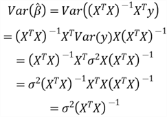
Therefore, when
 becomes significantly large, the variance of the
 is enormous.
We used the scatter plot matrix to detect linear relationships between pairs
of predictor variables. However, it is not easy to discover a multicollinear relationship
involving more than two predictor variables. We can use tolerance or Variance-inflation
factor (VIF) to detect multicollinearity (Jost, 2017). Before introducing the concepts
of tolerance and VIF, let us define
 .
We can construct a regression model when considering the
 predictor variable as the response variable, and all other predictors as predictor
variables. The R-squared of this model is
 .
We then can use
 to compute tolerance and VIF:

As a rule of thumb, if a value of tolerance is less than .20 (i.e., VIF is greater than 5.00), the model has a problem with multicollinearity. We use the following code to find the VIF of each predictor variable. The output of this script indicates "sqft_above"(VIF=5.394), "sqft_lot_log" (VIF=7.382), and "sqft_lot15_log" (VIF=7.088) have a multicollinear relationship with other predictor variables. We remove these predictor variables to re-run the following code. All VIF values in the second run are less than 5.0.
# The package contains the vif function
library(car)
full.model <- lm(price_log~bedrooms+bathrooms+sqft_lot_log+floors+
                   waterfront+view+condition+grade+
                   sqft_above+sqft_basement+yr_built+bln_renovated+
                   zipcode+lat+long+sqft_living15+
                   sqft_lot15_log, data=training.set.transform)
print(vif(full.model))
#output
#bedrooms    bathrooms   sqft_lot_log  floors         waterfront     view
#1.749261    3.279178    7.382354      2.330329       1.199954       1.402423
#condition   grade       sqft_above    sqft_basement  yr_built       bln_renovated
#1.284413    3.409414    5.394030      1.999548       2.375951       1.125687
#zipcode     lat         long          sqft_living15  sqft_lot15_log
#1.573033    1.255196    1.874210      3.110752       7.087844
3.6 Influential Points
We have observed outliers in Section 1.4.5. These outliers can also affect the OLS results. In some cases, a single point, usually an outlier in the predictor variables, can drastically change the parameter estimates. We call this point an influence point. Figure 8 demonstrates how an influence changes the slope of a simple regression line. This situation is undesirable because we want a regression model to represent all data points in a sample, not a few points. Therefore, to avoid this problem, data should meet the OLS assumption: larger outliers are unlikely (Hanck et al., 2020). It is worth noting that we should not automatically delete influence points because they might be the most critical points in the sample. Section 1.5 demonstrated that data transformation could reduce outliers.
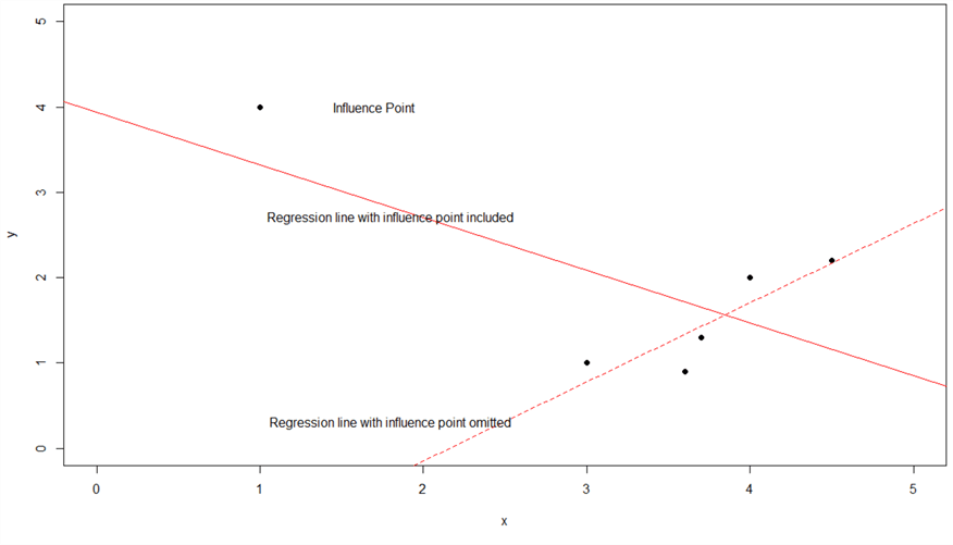
Figure 8 Effect of an Influential Point (Source: http://facweb.cs.depaul.edu/sjost/csc423/notes/influence-graph.png)
Professor Jost summarized five popular measures for identifying influence points (Jost, 2017):
- Externally Studentized Residual
- Leverage Statistic, or Hat-value
- Cook's D
- DFBETAS
- DFFITS
We can find free online resources that introduce the Externally Studentized Residual (PennState STAT 462) and Leverage Statistic measures (PennState STAT 501). In addition, the book that Montgomery and co-authors wrote introduces the measures Cook’s D, DFBETAS, and DFFITS (Montgomery et al., 2012). We have not discussed these measures in more depth in this exercise. Instead, we use the function "influence.measures()" in the car package to mark influence points with asterisks (*). This function prints the DFBETAS for each model variable, DFFITS, covariance ratios, Cook’s distances, and the diagonal elements of the hat matrix. The R function marks observations that are influential according to any of these measures with an asterisk. The following code demonstrates how to use this function:
 # The package contains the influence.measures function
library(car)
full.model <- lm(price_log~bedrooms+bathrooms+floors+waterfront+
                      view+condition+grade+sqft_basement+
                      yr_built+bln_renovated+zipcode+lat+
                      long+sqft_living15, data=training.set.transform)
print(influence.measures(full.model))
We should not simply discard these influential points. If an influential point is invalid, for example, recording error, it is appropriate to delete this point. Professor Jost introduced four possible remedies for influence points (Jost, 2017):
- Check for errors in the influential observations.
- Examine if the model does not include important independent variables.
- Apply a log or square root transformation to the predictor variables.
- Collect more data with predictor variables close to those of the influence points.
3.7 The Model Selection
A model may include all available predictor variables. We call this kind of model a full model. On the other hand, a null model is a model without any predictor variable. In practice, we often meet reduced models that do not include all possible predictor variables. For example, we removed four predictor variables and obtained a model with 14 predictor variables due to multicollinearity. All these 14 variables can construct 16,383 (=214-1) reduced models. Kadane and Lazar suggest using many tools to determine the best model (Kadane & Lazar, 2012). Different research areas may use different model selection criteria. Two commonly adopted selection criteria are adjusted R-squared and Akaike Information Criterion (AIC) (Sanquetta et al., 2018).
We discussed the adjected R-squared, which looks at whether additional predictor variables contribute to a model. When we add a set of predictor variables to a model, if the value of the adjusted R-squared becomes higher than the original one, this indicates that these additional variables are adding value to the model. Generally, when we add predictor variables to a null model, the adjusted R-squared value increases initially but decreases after it reaches the maximum. Thus, we can select a model with the highest value of the adjusted R-squared when using this selection criterion.
The AIC criterion, formulated by the statistician Hirotugu Akaike, measures the tradeoff between the uncertainty in a model and the number of predictor variables in the model (Jost, 2017). The best-fit model, according to AIC, is the one that explains the largest amount of variation in the response variable using the fewest possible predictor variables. It is worth noting that the AIC criterion measures model relatively. Therefore, we can only use the AIC scores to compare other AIC scores for the same dataset. A lower AIC score indicates a better model fit.
The best model is not always the most complicated one. Some variables may not be evidently important. We can use these three common model selection strategies to determine the best model:
- The backward selection strategy, which starts with a full model. For each variable in the current model, we investigate the effect of removing it. We then eliminate a variable that contributes the least information to the response variable. We eliminate a variable one at a time until the improvement is no longer statistically significant.
- The forward selection strategy, which is the reverse of the backward selection technique. We start with a null model. For each predictor variable not in the current model, we investigate the effect of including it. We include the most statistically significant variable not currently in the model. We repeat the process until we cannot find such a significant variable.
- The stepwise selection strategy, which is a combination of forward and backward selections. We start with a model, typically a null or full model; then, like the forward selection strategy, we add the most contributive predictor variable to the model. After adding a new variable, like backward selection, we eliminate any variables that no longer provide a statistically significant improvement in model fitting. We repeat the process until the model does not change.
The R language provides the "step()" function to implement these three strategies. When passing the values "backward," "forward," and "both" to the argument "direction," we can apply the backward, forward, and stepwise strategies, respectively. If we want to see information on each step, we can pass a TRUE value to the "trace" argument. The three strategies select the same regression model equation with 13 predictor variables. The adjusted R-squared has a value of 0.7493, and the Residual Standard Error, which is the square root of the residual sum of squares divided by the residual degrees of freedom, is 0.1127. However, this model may not be the best one when we take parsimony into account.
#1. Define null model.
null.model <- lm(price_log~1, data=training.set.transform)
#2. Define full model.
full.model <- lm(price_log~bedrooms+bathrooms+floors+waterfront+
                   view+condition+grade+sqft_basement+
                   yr_built+bln_renovated+zipcode+lat+
                   long+sqft_living15, data=training.set.transform)
#3. Perform backward selection:
cat("\nBackward Selection:\n")
step.backward <-step(full.model,
                     scope = list(lower = null.model, upper = full.model),
                     trace = TRUE,
                     direction="backward")
# Print out the summary
summary(step.backward)
#4. Perform forward selection:
cat("\nForward Selection:\n")
step.forward <-step(null.model,
                    scope = list(lower = null.model, upper = full.model),
                    trace = TRUE,
                    direction="forward")
# Print out the summary
summary(step.forward)
#5. Perform stepwise selection:
cat("\nStepwise Selection:\n")
step.stepwise <-step(null.model,
                     scope = list(lower = null.model, upper = full.model),
                     trace = TRUE,
                     direction="both")
# Print out the summary
summary(step.stepwise)
# The three strategies reach the same regression model equation
# Call:
#   lm(formula = price_log ~ grade + lat + sqft_living15 + yr_built +
#        bathrooms + view + floors + sqft_basement + zipcode + waterfront +
#        condition + bln_renovated + bedrooms, data = training.set.transform)
#
# Residuals:
#   Min       1Q   Median       3Q      Max
# -0.42887 -0.07162 -0.00326  0.06965  0.56726
#
# Coefficients:
#   Estimate Std. Error t value Pr(>|t|)
# (Intercept)     -1.979e+01  8.266e-01 -23.936  < 2e-16 ***
#   grade          7.675e-02  3.049e-03  25.174  < 2e-16 ***
#   lat            5.921e-01  1.631e-02  36.303  < 2e-16 ***
#   sqft_living15  7.484e-05  4.635e-06  16.146  < 2e-16 ***
#   yr_built      -1.830e-03  1.031e-04 -17.761  < 2e-16 ***
#   bathrooms      3.793e-02  4.659e-03   8.140 5.72e-16 ***
#   view           3.049e-02  3.134e-03   9.729  < 2e-16 ***
#   floors         5.124e-02  5.252e-03   9.756  < 2e-16 ***
#   sqft_basement  3.490e-05  5.916e-06   5.899 4.07e-09 ***
#   zipcode       -6.309e-04  1.253e-04  -5.034 5.08e-07 ***
#   waterfront     1.355e-01  2.636e-02   5.140 2.93e-07 ***
#   condition      1.875e-02  3.557e-03   5.270 1.46e-07 ***
#   bln_renovated  4.575e-02  1.109e-02   4.126 3.79e-05 ***
#   bedrooms       5.523e-03  2.900e-03   1.904    0.057 .
# ---
#   Signif. codes:  0 ‘***’ 0.001 ‘**’ 0.01 ‘*’ 0.05 ‘.’ 0.1 ‘ ’ 1
#
# Residual standard error: 0.1127 on 2988 degrees of freedom
# Multiple R-squared:  0.7504,Adjusted R-squared:  0.7493
# F-statistic:   691 on 13 and 2988 DF,  p-value: < 2.2e-16
3.8 External Model Validation
We already checked model adequacy using the overall F-test for regression and the adjusted R-squared. The regression model adequately fits the training data. However, a model we obtained from a sample may not successfully predict the values of the response variable based on new or future data points. The model validation involves an assessment of how the fitted model successfully makes a prediction. Therefore, we must assess the validity of the regression model in addition to its adequacy before using it in practice (Mendenhall & Sincich, 2012).
There are several model validation techniques. First, we can examine the predicted values. Suppose the predicted values do not make sense, for example, a negative value of the house sale price. In that case, we should re-visit the model fitting process. We also can examine the estimated coefficients if we have some prior knowledge of the model. For example, if we know that the older house would have a high sale price, the negative sign of the "yr_built" coefficient would be reasonable. The other techniques include collecting new data for prediction, cross-validation, and Jackknifing (Mendenhall & Sincich, 2012).
We collected a sample with size 6004, and we split the sample into training and
test datasets. We then used the training dataset to estimate the model parameters.
Now, we can use the test dataset to validate the model. The measure of model validity,
 ,
represents the percentage of variability in the test dataset explained by the model.
This measure is comparable to the R-squared in the model fitting process. We use
the following equation to calculate the measure:

The following R code computes the measure
 .
The value is 0.7645. Compared to the
 (=0.7504) from the training dataset, there is no significant drop but a slight increase.
This validation result increases our confidence in the model’s usefulness
(Mendenhall & Sincich, 2012).
 #1 Define the model.
fit.model <- lm(price_log~bedrooms+bathrooms+floors+waterfront+
                   view+condition+grade+sqft_basement+
                   yr_built+bln_renovated+zipcode+lat+
                   sqft_living15, data=training.set.transform)

#2, Obtain predicted values from test set.
p <- predict(fit.model, newdata=test.set.transform)
#3, Obtain residuals from test dataset.
r <- test.set.transform$price_log - p
#4, Obtain deviations
d <- test.set.transform$price_log - mean(test.set.transform$price_log)
#5, Calculate the measure.
r.sqaured.prediction <- 1- sum(r^2)/sum(d^2)
r.sqaured.prediction
#[1] 0.7644722
4 – Specifying the Error Term Distribution and Estimating its Variance
We hypothesized the form of multiple linear regression:

The error term
 (or disturbance) is a theoretical concept that measures the difference between the
observed values for the response variable and its theoretical values according to
the model. Since the parameter
 is unknown, we cannot observe (or calculate) the error term (Carlos, 2013). Nevertheless,
the error term plays a major role in regression analysis.
4.1 The Gauss-Markov Assumptions
To use the OLS method to perform model fitting, we have four assumptions. The method can perform well when sample data meets all these assumptions. Since we use sample data to compute the estimators, we should make statistical inferences to draw conclusions about the underlying population. According to the Gauss-Markov theorem, we can obtain the best linear unbiased estimators through the OLS method when the model meets the first six Gauss-Markov assumptions:
- Linearity in parameters:

- The expected value of the error term is zero:

- The variance of the error term is a constant:

- The error term is independently distributed and uncorrelated:

- Any predictor variable is uncorrelated to the error term:

- The design matrix
 is an
is an
 matrix of full rank (or no perfect multicollinearity).
 - The error term has a normal distribution:

The last assumption makes hypothesis testing easier. However, the Gauss-Markov Theorem does not require that the error term has a normal distribution. When the sample size is large, the law of large numbers and the central limit theorem come to justify the assumption. Thus, even if the error term violates the "normality assumption" rule, the OLS estimators still have approximately normal distributions.
Regression analysis does not require a model to meet all these assumptions. Depending
on how we use the model, the model requires different assumptions. For example,
suppose we are only interested in an unbiased estimate of
 .
In that case, the assumptions about the variance or the covariance of the error
terms
 are not required (Rothman, 2020). We prove this in Section
4.2.
Therefore, it is not always necessary to check all these seven assumptions. Many
texts make four basic assumptions about the error terms ε (Mendenhall &
Sincich, 2012):
- Unbiasedness:

- Homoscedasticity:

- Independence:

- Normality:

In other words, the errors,
 ,
should be independent normal random variables with mean zero and constant variance,
 .
The following section uses these assumptions to make statistical inferences.
4.2 Statistical Inference
The validity of many statistical inferences associated with a regression analysis
depends on the error term satisfying these assumptions. Based on the Gauss-Markov
assumptions, we can prove that
 is an unbiased estimator of
 and construct confidence intervals on regression coefficients, the mean response,
and predictions.
We write the equation to compute the regression coefficient estimator and Gauss-Markov assumption 1:


Therefore,

Then, using the properties of the expected value (Taboga, 2017), we compute the expected value of the estimator using the assumption 5:

According to assumption 2,
 ,
we then have this equation:

Thus, if assumptions 1, 2 and 5 are satisfied, we can say that
 is an unbiased estimator of
 (Adhikari, 2021). Furthermore, we can conclude that the difference between residuals
and error term has an expected value of zero:

Assumption 3 states that the variance of the error term,
 ,
is constant but unknown. However, the literature (Montgomery et al., 2012) proves
that the expected value of MSE is
 ;
therefore, an unbiased estimator of
 can be computed by this formula:

In this exercise, we consider that the predictor variables have fixed values. According to assumptions 3 and 4, each error term is uncorrelated and has the same variance. Moreover, for independent random variables, the variance of their sum or difference is the sum of their variances. As a result, we can obtain the variance of the response variable (Seber & Lee, 2003):
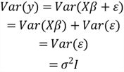
Now, we can find the variance of the estimator
 :
:
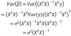
The term
 ,
denoted by
 ,
is a
 symmetric matrix, in which the diagonal element
 is the variance of
 .
The off-diagonal element, such as
 ,
is the covariance between
 and
and
 .
The variance-covariance matrix has this form:

Consequently, when we know the value of
 ,
we can calculate the standard error of the regression coefficient
 :
:

Then, we can obtain a 100(1-α) percent confidence interval for the regression
coefficient
 :
:

We also can construct a confidence interval for the mean response at a given
data point, for example
 .
The estimator of the response variable, given
 ,
is
,
is

Then, we can obtain the variance of
 :
:
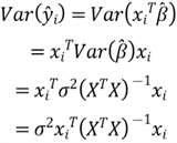
Therefore, we can calculate the 100(1-α) percent confidence interval for
the mean response at a given data point
 :
:

Note that this confidence interval is not appropriate for predicting a future
observation, for example
 .
The future observation has a variance
 and is independent of the estimator. Therefore,
 is normal distributed with mean zero and variance:
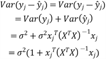
Therefore, we can calculate the 100(1-α) percent prediction interval for
the future observation at the data point
 :
:

5 – Evaluating the Utility of the Model
We performed the overall F-test for regression in Section 3.3. The test checked the null hypothesis that there is no useful linear relationship between the response variable and any predictor variables. We rejected the null hypothesis; therefore, we have sufficient evidence to support that at least one of these predictor variables is related to the response variable. We then determined that the model was useful.
Section 3.7 selected a model, and the R tool automatically conducted a series of t-tests to determine model adequacy. However, for a model with many predictor variables, we should avoid conducting t-tests. Instead, we should rely on the global F-test and partial F-tests to determine which specific regressors seem important to the response variables (Mendenhall & Sincich, 2012). Therefore, this section explores the three types of multiple linear regression parameter tests.
5.1 A Limitation of the T-test
When performing the simple linear regression analysis, we conducted a t-test
on the unknown parameter,
 (Zhou, 2020). The null hypothesis is that the unknown parameter,
 ,
is zero. We reject the null hypothesis if we find the result of a test procedure
is unlikely when the null hypothesis is true. However, a type I error occurs if
we reject the null hypothesis when it is true. The probability of this error is
the type I error rate (also known as the significance level), denoted by α.
We usually set α to 0.05(5%). This level indicates we can accept a 5% chance
of incorrectly rejecting the true null hypothesis. Therefore, even though the response
variable and the predictor variable do not have a linear relationship, we have a
5% chance of rejecting that the parameter is zero.
Suppose that we have a multiple linear regression model that has two predictor variables:

There are four possible outcomes when we study the significance of the unknown
parameters
 and
and
 :
:


Assuming the response variable does not have any relationship with these two predictor variables. In this case, the Venn diagram, Figure 9, illustrates the chance that at least one parameter is not zero:
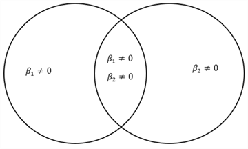
Figure 9 The chance of at least one parameter not being zero given no relationship between the response and predictors
If α = 0.05, we calculate the chance of at least one parameter not being zero when the null hypothesis is true:

Therefore, the overall type I error is 0.975, not 0.05. When we have 13 predictor variables, the overall type I error increases significantly:

Suppose the response variable does not have any relationship with these 13 predictor variables. In that case, the t-test on the model's all 13 parameters implies an approximately 48.7% chance of incorrectly concluding that some parameters are not zero. It is worth noting that the t-test is a partial test because the test checks the contribution of one predictor variable, given the other predictors in the model. Therefore, the t-test does not work for hypotheses involving multiple regression models with many predictor variables. Instead, we use F-test to evaluate hypotheses that involve multiple parameters.
5.2 The Partial F-test
Assuming we have a regression model:

We arrange the p unknown parameters into two groups:

 and
and
 represent two vectors of the regression coefficients. We re-write the model in this
form:

Then, we want to test the hypotheses:

If the null hypothesis is true, we have this model:

This model contains a subset of the predictor variables in the overall regression
model. We call this model a nested (or reduced) model, and call the overall regression
model a full model (or complete). By comparing a reduced model with the full model,
we can assess the usefulness of predictors in the vector
 .
Therefore, this test determines if the full model and the nested model are significantly
different. Because this test measures the contribution of the regressors in
 given that the other regressors in
 are in the model, some authors call the test a partial F test (Montgomery et al.,
2012). We define the test statistic as the follows (Mendenhall & Sincich, 2012):
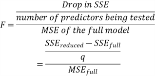
When the reduced model is a null model, the residual sum of squares of the reduced model equals to the sum of squares total. Therefore, the F-test statistic calculation here agrees with the formula in Section 3.3, where we conducted the overall F-test for regression. Similarly, we can apply the five-step process to conduct a partial F-test. The subsequent sections conduct partial F-tests to answer three research questions (PennState STAT 462):
- Does the regression model contain at least one predictor useful in predicting the sales price of a house?
- Does the price significantly (linearly) relate to the number of bedrooms in the house?
- Does the price significantly (linearly) relate to the geographic location, i.e., the zip code and the latitude?
5.3 Testing All Parameters Equal to Zero
To answer the research question: "Does the regression model contain at least one predictor useful in predicting the sales price of a house?" we test the hypotheses:

The full model that contains all 13 predictor variables is in this form:

We then construct the reduced model that does not contain any predictor variables:

Rather than flowing the five-step process to conduct the F-test manually, we can use the following R script to conduct the partial F-test. Since p-value: < 2.2e-16, we reject the null hypothesis. There is sufficient evidence to conclude that at least one predictor is useful in predicting the sales price of a house. Using the R function "summary()," we can see that the anova() function and the lm() function produce the same results as the t-test. This F-test has various names such as "model utility test," "overall F-test," and "F-test for regression relation."
#1, Define the reduced model (i.e., the null model).
null.model <- lm(price_log~1, data=training.set)
#2, Define the full model.
full.model <- lm(price_log~bedrooms+bathrooms+floors+waterfront+
                  view+condition+grade+sqft_basement+
                  yr_built+bln_renovated+zipcode+lat+
                  sqft_living15, data=training.set.transform)
#3, Compare the null.model to the full model
anova(null.model, full.model)
#Output
# Analysis of Variance Table
#
# Model 1: price_log ~ 1
# Model 2: price_log ~ bedrooms + bathrooms + floors + waterfront + view +
#   condition + grade + sqft_basement + yr_built + bln_renovated +
#   zipcode + lat + sqft_living15
# Res.Df     RSS Df Sum of Sq      F    Pr(>F)
# 1   3001 152.114
# 2   2988  37.968 13    114.15 691.01 < 2.2e-16 ***
#   ---
#   Signif. codes:  0 ‘***’ 0.001 ‘**’ 0.01 ‘*’ 0.05 ‘.’ 0.1 ‘ ’ 1
5.4 Testing One Parameter Equal to Zero
To answer the research question: " Does the price significantly (linearly) relate to the number of bedrooms in the house?" we test the hypotheses:

The full model contains all 13 predictor variables. The reduced model is a special case of the full model. By setting the testing coefficient to zero, we obtain the reduced model:

We use the following R script to conduct the partial F-test. Since p-value: > 0.05, we fail to reject the null hypothesis. We have insufficient evidence to say that the price significantly (linearly) relates to the number of bedrooms in the house. We adopt the principle of parsimony; we eliminate the "bedrooms" variable in the model even though we do not know the Type II error.
#1, Define the reduced model.
reduced.model <- lm(price_log~bathrooms+floors+waterfront+view+
                      condition+grade+sqft_basement+yr_built+
                      bln_renovated+zipcode+lat+sqft_living15,
                    data=training.set.transform)

#2, Define the full model.
full.model <- lm(price_log~bedrooms+bathrooms+floors+waterfront+
                   view+condition+grade+sqft_basement+
                   yr_built+bln_renovated+zipcode+lat+
                   sqft_living15, data=training.set.transform)

#3, Compare the null.model to the full model
anova(reduced.model, full.model)
#Output
# Analysis of Variance Table
#
# Model 1: price_log ~ bathrooms + floors + waterfront + view + condition +
#   grade + sqft_basement + yr_built + bln_renovated + zipcode +
#   lat + sqft_living15
# Model 2: price_log ~ bedrooms + bathrooms + floors + waterfront + view +
#   condition + grade + sqft_basement + yr_built + bln_renovated +
#   zipcode + lat + sqft_living15
# Res.Df    RSS Df Sum of Sq      F  Pr(>F)
# 1   2989 38.014
# 2   2988 37.968  1  0.046084 3.6267 0.05695 .
# ---
#   Signif. codes:  0 ‘***’ 0.001 ‘**’ 0.01 ‘*’ 0.05 ‘.’ 0.1 ‘ ’ 1
We can use the function "summary ()" to look at the t-test on the "bedrooms" variable. The p-value for the t-test on the bedrooms is the same as the p-value we obtained from the partial F-test. We also noticed that the F- statistic, i.e., 3.6267, approximates the square of the t- statistic (i.e.,1.904X1.904=3.625). Thus, when we test whether only one parameter is zero, there is a relationship between the t-statistic and F-statistic:

Therefore, we can use either the F-test or the t-test to check if one coefficient is zero given other predictors in the model.
5.5 Testing a Subset of Parameters Equal to Zero
To answer the research question: "Does the price significantly (linearly) relate to the geographic location, i.e., the zip code and the latitude?" we test the hypotheses:

We eliminated the "bedrooms" variable; therefore, the full model contains all 12 predictor variables in this test:

We then construct the reduced model that does not contain the predictor variables, the zip code, and the latitude:

We can use the following R script to conduct the partial F-test. The F-statistic is 670.18. If the null hypothesis is true, the probability of observing such the F-statistic is less than the p-value, i.e., 2.2e-16. Therefore, obtaining the F-statistic is extremely unlikely. Thus, we reject the null hypothesis. In this case, we have sufficient evidence to conclude that the geographic location significantly (linearly) relates to the price.
#1, Define the reduced model.
reduced.model <- lm(price_log~bathrooms+floors+waterfront+view+
                      condition+grade+sqft_basement+yr_built+
                      bln_renovated+sqft_living15,
                    data=training.set.transform)
#2, Define the full model.
full.model <- lm(price_log~bathrooms+floors+waterfront+view+
                   condition+grade+sqft_basement+yr_built+
                   bln_renovated+zipcode+lat+sqft_living15,
                 data=training.set.transform)
#3, Compare the null.model to the full model
anova(reduced.model, full.model)

# Output
# Analysis of Variance Table
#
# Model 1: price_log ~ bathrooms + floors + waterfront + view + condition +
#   grade + sqft_basement + yr_built + bln_renovated + sqft_living15
# Model 2: price_log ~ bathrooms + floors + waterfront + view + condition +
#   grade + sqft_basement + yr_built + bln_renovated + zipcode +
#   lat + sqft_living15
# Res.Df    RSS Df Sum of Sq      F    Pr(>F)
# 1   2991 55.076
# 2   2989 38.014  2    17.063 670.81 < 2.2e-16 ***
#   ---
#   Signif. codes:  0 ‘***’ 0.001 ‘**’ 0.01 ‘*’ 0.05 ‘.’ 0.1 ‘ ’ 1
6 – Checking Model Adequacy
The inferential analysis in Section 4.2 indicates that these inferences depend on whether the error term meets certain assumptions. Therefore, to complete a regression analysis, we should examine whether the errors meet these assumptions. Experience has shown that OLS regression analysis can produce reliable confidence intervals and statistical test results if the error term does not significantly depart from these assumptions (Mendenhall & Sincich, 2012).
6.1 Residual Analysis
We have already seen the following two regression equations. By re-arranging
these two equations, we can obtain the definitions of the error term
 and the residuals
 :
:
- Population regression equation:

- Sample regression equation:

The error term
 is unknown, but the residuals are known. The following derivation helps to discover
the relationship between
 and
and
 :
:
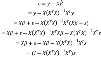
Therefore, the residuals
 are a linear combination of the error term
 .
Subtracting the two regression equations, we obtain the difference between the residuals
and the error term:

The difference between them has an expected value of zero:

Section 3.2 demonstrated two properties of residuals:


where s denotes the standard deviation of the residual, which is equal to the standard deviation of the fitted regression model.
Since the error term is unknown, we use the residuals to estimate its values (Mendenhall & Sincich, 2012). It is convenient to think of the residuals as the realized or observed values of the model errors. According to the properties of residuals, any departures from the assumptions on the errors should show up in the residuals (Montgomery et al., 2012). Thus, we perform residual analysis, a mathematical method for checking if the model is a good fit. We often examine residual plots to investigate model fitting and check the assumptions. A careful graphical analysis of residuals is essential for regression analysis (Chatterjee & Hadi, 2006).
We have covered the four basic assumptions in Section 4.1, i.e., Unbiasedness, Homoscedasticity, Independence, and Normality. The residuals are not independent because the n residuals have only (n–p-1) degrees of freedom associated with them. However, this non-independence of the residuals has little effect on checking model adequacy if n is not small relative to the number of parameters p (Montgomery et al., 2012). We use residual plots to check other three basic assumptions:
- Unbiasedness: Examine the residual plots of the residuals vs. the predictor variables or residuals vs. the predicted values. In each plot, look for trends, dramatic changes in variability, or more than 5% of residuals that lie outside two estimated standard deviations of zero. Any of these patterns indicate a violation of the unbiasedness assumption (Mendenhall & Sincich, 2012).
- Homoscedasticity: Examine the residual plots of the residuals vs. the predictor variables or residuals vs. the predicted values. The standard deviation of the residuals is the same in any thin rectangle in the residual plot.
- Normality: Examine the normal Q–Q (quantile-quantile) plot. In the plot, the observed points (dots) should be around the diagonal line.
6.2 Residual Plots
Even though we can perform formal statistical tests to investigate model adequacy and check model assumptions, it is convenient to inspect residuals visually. Residual plots are helpful to check the unbiasedness and homoscedasticity assumptions. A residual plot, which is a scatter diagram, plots the residuals on the y-axis vs. the fitted values on the x-axis. We can also produce residual plots of the residuals vs. a single predictor variable. When a regression model satisfies the unbiased and homoscedastic assumptions, its residual plot should have a random pattern.
Additionally, we can create a normal probability plot of the residuals to check the normality assumption. The normal probability plot, a graphical technique, can check the normality assumption. We usually see two kinds of probability plots: Q-Q and P-P. In this exercise, we adopt the Q-Q plot, a scatter diagram of the empirical quantiles of the residuals (y-axis) against the theoretical quantiles of a normal distribution (x-axis). If the Q-Q plot is close to a straight line, the residuals' probability distribution is close to normal.
6.2.1 Check the Unbiasedness and Homoscedasticity Assumptions
A plot of the residuals vs. the corresponding fitted values or individual predictor variable helps detect several common types of model inadequacies. Professor Jost summarized six patterns of residual plots (Jost, 2017), shown in Figure 10. If the plot has a random pattern, as illustrated in graph (a), the residuals are in a horizontal band; therefore, there are no obvious model defects. However, the other patterns are symptomatic of model deficiencies. For example, the model may miss some predictors, or the linear model may not be the best technique for the data under analysis (Frost, 2017).
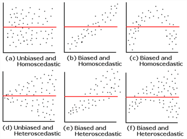
Figure 10 Professor Jost's six patterns of residual plot (Jost, 2017)
We have already determined a multiple linear regression model using R. We use the following script to produce residual plots, as shown in Figure 11. For demonstration purposes, we produced four plots: (a) residuals vs. fitted values; (b) residuals vs. the "sqlt_living15" variable; (c) residuals vs. the "yr_built" variable; and (d) residuals vs. the "lat" variable. The pattern in the residual plots (a), (b), and (c) is approximately random. However, plot (c) shows a curve in the residual plot. Comparing to Professor’s six patterns, we can see the residuals are biased and homoscedastic. The curve indicates a non-linear relationship in the original dataset. We may add a squared term to get the plot randomly scattered without any trend (Kim, 2019). This article aims to introduce the basic steps to perform multiple regression analysis. Future studies will focus on the remedies for assumption violations.
# Use the 'gridExtra' library.
# Store each plot and then use the grid.arrange command
# which lets you specify number of rows and columns of graphs
library(gridExtra)

#1, Define the final model.
fit.model <- lm(price_log~bathrooms+floors+waterfront+view+
                  condition+grade+sqft_basement+yr_built+
                  bln_renovated+zipcode+lat+sqft_living15,
                data=training.set.transform)
#2 Get residuals
training.set.transform$residual <- residuals(fit.model)
#3 Get fitted values
training.set.transform$fitted <- fitted(fit.model)
# Produce residual plots
p1<-ggplot(data = training.set.transform, aes(x=fitted, y=residual)) +
  geom_point()+
  geom_hline(yintercept=0, col="red", linetype="dashed") +
  xlab("Fitted values")+
  ylab("Residuals") +
  ggtitle("(a), Residuals vs. Fitted Values") +
  theme_bw() +
  theme(plot.title = element_text(hjust = 0.5,size=18),
        axis.title = element_text(size=14),
        axis.title.x = element_text(margin = margin(t = 5, r = 0, b = 0, l = 0)))
p2<-ggplot(data = training.set.transform, aes(x=sqft_living15, y=residual)) +
  geom_point()+
  geom_hline(yintercept=0, col="red", linetype="dashed") +
  xlab("sqft_living15")+
  ylab("Residuals") +
  ggtitle("(b), Residuals vs. sqft_living15 Variable") +
  theme_bw() +
  theme(plot.title = element_text(hjust = 0.5,size=18),
        axis.title = element_text(size=14),
        axis.title.x = element_text(margin = margin(t = 5, r = 0, b = 0, l = 0)))
p3<-ggplot(data = training.set.transform, aes(x=yr_built, y=residual)) +
  geom_point()+
  geom_hline(yintercept=0, col="red", linetype="dashed") +
  xlab("yr_built")+
  ylab("Residuals") +
  ggtitle("(c), Residuals vs. yr_built Variable") +
  theme_bw() +
  theme(plot.title = element_text(hjust = 0.5,size=18),
        axis.title = element_text(size=14),
        axis.title.x = element_text(margin = margin(t = 5, r = 0, b = 0, l = 0)))
p4<-ggplot(data = training.set.transform, aes(x=lat, y=residual)) +
  geom_point()+
  geom_hline(yintercept=0, col="red", linetype="dashed") +
  xlab("lat")+
  ylab("Residuals") +
  ggtitle("(d), Residuals vs. lat Variable") +
  theme_bw() +
  theme(plot.title = element_text(hjust = 0.5,size=18),
        axis.title = element_text(size=14),
        axis.title.x = element_text(margin = margin(t = 5, r = 0, b = 0, l = 0)))
# Put them in 2 columns
grid.arrange(p1,p2,p3,p4,ncol=2)
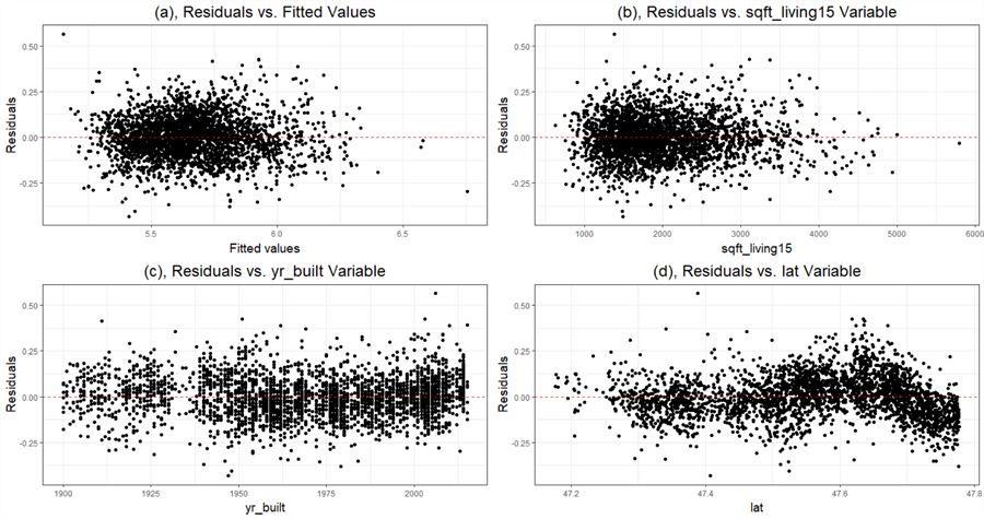
Figure 11 Residual Plots
6.2.2 Check Normality Assumption
Statistical inferences such as hypothesis tests, parameter confidence intervals, and prediction confidence intervals depend on the normality assumption. However, slight departures from the normality assumption do not affect the model significantly (Montgomery et al., 2012). Professor Jost provided sketches of five normal plots and their interpretations (Jost, 2017), shown in Figure 12. We can compare the normal plot we obtained to these sketches and then decide what remedial measures we should apply, if any. We should pay more attention to those error distributions with thicker or heavier tails. These thicker or heavier tails indicate that the OLS method may be sensitive to a small amount of data.
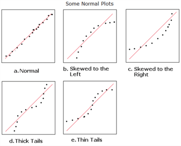
Figure 12 Professor Jost's five patterns of normal plot (Jost, 2017)
The following script can produce a Q-Q plot, as shown in Figure 13. The Q-Q plot indicates that the residual distribution has thick tails. Therefore, residuals have more extreme values than expected if they have a normal distribution. Accordingly, when residuals do not have a normal distribution, we should apply some methods to rectify the model (Barker & Shaw, 2015). However, the normality assumption is the least restrictive when applying regression analysis in practice (Mendenhall & Sincich, 2012). Therefore, when the departures from the normality assumption are moderate, such departures have minimal effect on the statistical tests and the confidence interval constructions.
#1, Define the final model.
fit.model <- lm(price_log~bathrooms+floors+waterfront+view+
                  condition+grade+sqft_basement+yr_built+
                  bln_renovated+zipcode+lat+sqft_living15,
                data=training.set.transform)
#2 Get residuals
training.set.transform$residuals <- residuals(fit.model)
#3 Produce q-q plot
ggplot(training.set.transform, aes(sample=residuals)) +
  geom_qq() +
  # adding the line for comparison against perfect fit is done with a separate layer
  geom_qq_line()  +
  xlab("theoretical")+
  ylab("sample") +
  theme_bw() +
  theme(plot.title = element_text(hjust = 0.5,size=18),
        axis.title = element_text(size=14),
        axis.title.x = element_text(margin = margin(t = 5, r = 0, b = 0, l = 0)))
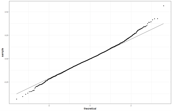
Figure 13 The Normal Q-Q Plot
7 – Applying the Model
We used the model selection strategy to select a model, conducted F-tests to eliminate an insignificant variable, and performed residual analysis. We found a model with 12 predictor variables. The adjusted R-squared is 0.75, which implies that the model could explain 75% of the variance in the response variable. Therefore, this model is acceptable. Table 2 illustrates the estimated coefficients. We then use the model to solve the business requirements in the problem statements. We often use the model to interpret the relationship between the response variable and the predictor variables, estimate the response variable's mean value, and make predictions.
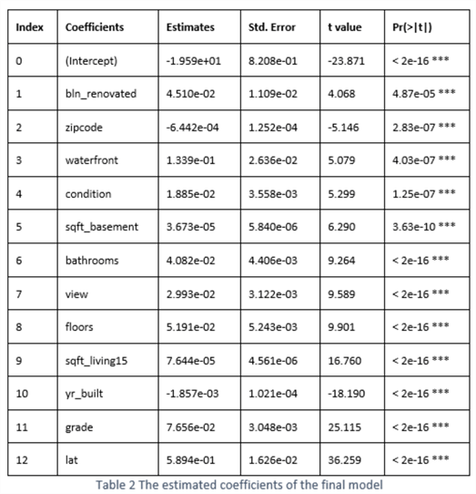
7.1 Interpreting the Model
We used a multiple regression model to describe the relationship between the response variable and the predictor variables:

The parameter
 indicates the expected change in the response variable(y) per unit change in
 when all other predictor variable is held constant. For example, the mean increase
of the response variable is 0.0451 when a house is renovated. Another example is
that the mean of the response variable decreases by 0.00196 if the built year increases
by one year. Since we applied the logarithm to the response variable, "price",
we rewrite the model equation:

We observe that the predictor variable and error term enter the model multiplicatively
instead of additively. As a result, the interpretation of unit change in predictor
variables is different. For example, with all other predictors holding constant,
changing a house from non-renovated to renovated increases the price by 10.9% ( ).
Similarly, if the built year increases by one year, the price decreases 0.44% (
 ).
).
7.2 Using the Model for Estimation
When repeating an experiment many times, we can observe that the response variable is a random variable. Furthermore, we assumed that the response variable at any data point has an independent and identical distribution. Therefore, with the model, we can estimate the mean value of the response variable when given a data point:

The following R scripts select a data point and then obtain the mean response
and the 95% confidence interval at the data point. For example, the program picks
up a data point
 .
The output shows that the mean response is 5.498, and the 95% confidence interval
is [5.486, 5.510]. Therefore, when given the selected data point
 ,
we are 95% confident that the true mean is between 5.486 and 5.510. It is noteworthy
that we obtained this confidence interval on the transformed response variable.
We do not recommend the use of reverse transformations to get the confidence interval
of the original scale (Pek et al., 2017).
#1, Define the final model.
fit.model <- lm(price_log~bathrooms+floors+waterfront+view+
                  condition+grade+sqft_basement+yr_built+
                  bln_renovated+zipcode+lat+sqft_living15,
                data=training.set.transform)
#2, Randomly pick a data point
set.seed(314)
data.point <- training.set.transform[sample(nrow(training.set.transform), 1), ]
#3, Estimate a mean response
predict(fit.model, newdata = data.point, interval ="confidence")
#output
#fit      lwr      upr
#5.497991 5.486249 5.509734
7.3 Using the Model for Prediction
Suppose a homeowner wants to sell his/her house. In that case, we can use the
model to predict a particular sales price for given house characteristics. In other
words, we predict the outcome of a single experiment at a given data point. As mentioned
in Section
4.2, the new observation has a variance of
 ,
and it is independent of the estimator of the response variable. Therefore, we use
different equations to compute the prediction interval, as shown in Section
4.2.
We use the following R script to obtain the predicted value of the response variable and 95% prediction interval. At the given data point, the predicted value is 5.498; and the 95% prediction interval is [5.277, 5.719]. The predicted value is the same as the mean response, given the same data point; however, the interval is wider. When constructing the prediction interval, we need to be concerned about two errors: the error of estimating the mean response, and the error of the predicted value. Therefore, the predicted value is more uncertain than the mean response. Because the confidence interval gives more information about the population than the prediction interval, we often use the confidence intervals to represent data.
#1, Define the final model.
fit.model <- lm(price_log~bathrooms+floors+waterfront+view+
                  condition+grade+sqft_basement+yr_built+
                  bln_renovated+zipcode+lat+sqft_living15,
                data=training.set.transform)
#2, Randomly pick a data point
set.seed(314)
data.point <- training.set.transform[sample(nrow(training.set.transform), 1), ]
#3, Make a prediction
predict(fit.model, newdata = data.point, interval ="prediction")
# output
# fit      lwr      upr
# 5.497991 5.276558 5.719425
8 – Conclusion
We explored the seven-step procedure to build a multiple linear regression model. We covered two essential parts of regression analysis when walking through the process: exploratory data analysis and residual analysis. We also covered fundamental techniques such as OLS, data transformation, F-test, multicollinearity, influential points, model selection strategy and model validation. Besides providing R scripts to implement the process, the article provided mathematical derivations to explain these statistical techniques and the analysis process.
After defining the problem statements, we started to introduce techniques for data collection and data examination. Next, we hypothesized a form of the multiple linear regression model. The model contained unknown parameters. We then used the OLS technique to estimate these unknown parameters. Next, we discussed the backward, forward, and stepwise model selection strategies; and used these strategies to select a model. We then presented the Gauss-Markov assumptions and four basic assumptions. The mathematical derivations implied that the statistical inferences, such as confidence intervals and statistic tests, depended on these assumptions. Therefore, violations of these assumptions might cause model deficiencies.
We conducted F-tests to evaluate the model utility, and performed residual analysis to check model adequacy. After going through all these steps, we obtained an acceptable model. With the model, we interpreted the relationships between the sales price and the house characteristics. Then, when given house characteristics, we used the model to estimate the mean price value and predict the price.
Reference
Adhikari, A. (2021). Unbiased Estimators. http://stat88.org/textbook/notebooks/Chapter_05/04_Unbiased_Estimators.html
Alexander, R. (2021). Telling Stories with Data. https://www.tellingstorieswithdata.com.
Banjar, H., Ranasinghe, D., Brown,F., Adelson, D., Kroger,T., Leclercq,T., White,D.,Hughes,T. and Chaudhri,N. (2017). Modelling Predictors of Molecular Response to Frontline Imatinib for Patients with Chronic Myeloid Leukaemia. PLoS One, vol. 12, no. 1, Public Library of Science, Jan. 2017, p. e0168947.
Barker, L. E., & Shaw, K. M. (2015). Best (but oft-forgotten) practices: checking assumptions concerning regression residuals. The American journal of clinical nutrition, 102(3), 533–539. https://doi.org/10.3945/ajcn.115.113498.
Birkett, A. (2019). How to Deal with Outliers in Your Data. https://cxl.com/blog/outliers.
Carlos, Á. F. (2013). Re: What is the difference between error terms and residuals in econometrics (or in regression models)?. https://www.researchgate.net/post/What_is_the_difference_between_error_terms_and_residuals_in_econometrics_or_in_regression_models/.
Chang, W. (2018). R Graphics Cookbook: Practical Recipes for Visualizing Data 2nd Edition. https://r-graphics.org/
Chatterjee, S., & Hadi, S. A. (2006). Regression Analysis by Example, 4th Edition. Hoboken, NJ: Wiley.
Chin, W. W. (1998). The partial least squares approach for structural equation modeling. Mahwah, NJ: Lawrence Erlbaum Associates.
Davidson, J. (2018). An Introduction to Econometric Theory. Hoboken, NJ: Wiley.
Dong, X. (2012). whisker of boxplot. https://www.r-bloggers.com/2012/06/whisker-of-boxplot/.
Espinoza, J. J. (2012). The Least Squares Assumptions, https://masterofeconomics.org/2012/07/18/the-least-squares-assumptions.
Finnstats. (2021). A Brief Introduction to ggpairs. https://www.r-bloggers.com/2021/06/ggpairs-in-r-a-brief-introduction-to-ggpairs/.
Frost, J. (2017). Check Your Residual Plots to Ensure Trustworthy Regression Results!. https://statisticsbyjim.com/regression/check-residual-plots-regression-analysis/.
Frost, J. (2018). How to Interpret the Constant (Y Intercept) in Regression Analysis. https://statisticsbyjim.com/regression/interpret-constant-y-intercept-regression.
Frost, J. (2018). How to Choose Between Linear and Nonlinear Regression. https://statisticsbyjim.com/regression/choose-linear-nonlinear-regression.
Frost, J. (2018). How To Interpret R-squared in Regression Analysis. https://statisticsbyjim.com/regression/choose-linear-nonlinear-regression/.
Gallo, A. (2015). A Refresher on Regression Analysis. https://hbr.org/2015/11/a-refresher-on-regression-analysis.
Garrett, C. (2020). Data on the Edge: Handling Outliers. https://www.rapidinsight.com/blog/handle-outliers.
Han, J., Kamber, M. & Pei, j. (2012). Data Mining Concepts and Techniques. Waltham, MA: Morgan Kaufmann.
Hanck, C., Arnold, M., Gerber. A., & Schmelzer, M. (2020). Introduction to Econometrics with R. https://www.econometrics-with-r.org.
Harlfoxem (2016), House Sales in King County, USA. https://www.kaggle.com/harlfoxem/housesalesprediction.
Holmes, A., Illowsky, B., Dean, S., & Hadley, k. (2017). Introductory Business Statistics. https://openstax.org/details/books/introductory-business-statistics.
Kim, H. Y. (2019). Statistical notes for clinical researchers: simple linear regression 3 – residual analysis. https://rde.ac/DOIx.php?id=10.5395/rde.2019.44.e11.
IBM Cloud Education. (2020). Exploratory Data Analysis. https://www.ibm.com/cloud/learn/exploratory-data-analysis.
Ismay, C., & Kim, Y. A. (2021). Statistical Inference via Data Science: A ModernDive into R and the Tidyverse. https://moderndive.com/.
Johnson, P. W. & Myatt, J. G. (2014). Making Sense of Data I: A Practical Guide to Exploratory Data Analysis and Data Mining, 2nd Edition. Hoboken, NJ: Wiley.
Jost, S. (2017). CSC 423: Data Analysis and Regression Lecture Note. http://facweb.cs.depaul.edu/sjost/csc423/.
Kadane, J.B.& Lazar, N.A. (2012) Methods and criteria for model selection. Journal of the American Statistical Association. https ://doi.org/10.1198/016214504000000269.
Kiernan, D. (2014). Natural Resources Biometrics. https://open.umn.edu/opentextbooks/textbooks/205.
Kumar, S. (2020). 7 Ways to Handle Missing Values in Machine Learning. https://towardsdatascience.com/7-ways-to-handle-missing-values-in-machine-learning-1a6326adf79e
Li, X., Wong, W., Lamoureux, L. E. & Wong, Y. T. (2012). Are Linear Regression Techniques Appropriate for Analysis When the Dependent (Outcome) Variable Is Not Normally Distributed? Investigative Ophthalmology & Visual Science May 2012, Vol.53, 3082-3083. doi: https://doi.org/10.1167/iovs.12-9967.
Liu, J. (2020). In a linear model, Sum of Squared Regression(SSR) may stay unchanged or increase as predictors are added to a regression model. https://www.quora.com/Linear-Models-Why-does-regression-sum-of-squares-increase-as-predictors-are-added-to-a-regression-model
Mazza-Anthony, C. (2021). A Five-Step Guide for Conducting Exploratory Data Analysis, https://shopify.engineering/conducting-exploratory-data-analysis
Mendenhall, W., & Sincich, T. (2012). A Second Course in Statistics: Regression Analysis (7th Edition). Boston, MA: Prentice Hall.
Montgomery, C. D., Peck A. E. & Vining, G. G. (2012). Introduction to Linear Regression Analysis (5th Edition). Hoboken, NJ: Wiley.
Osborne, J. (2002). Notes on the use of data transformations. Practical Assessment, Research & Evaluation, 8(6). https://scholarworks.umass.edu/pare/vol8/iss1/6/.
Pasta. J. D. (2009). Learning When to Be Discrete: Continuous vs. Categorical Predictors. ICON Clinical Research, San Francisco, CA, http://support.sas.com/resources/papers/proceedings09/248-2009.pdf.
Pek, J.; Wong, O., & Wong, A. C. (2017) "Data Transformations for Inference with Linear Regression: Clarifications and Recommendations," Practical Assessment, Research, and Evaluation: Vol. 22, Article 9. DOI: https://doi.org/10.7275/2w3n-0f07 Available at: https://scholarworks.umass.edu/pare/vol22/iss1/9.
Redman, C. T. (2008). Data Driven: Profiting from Your Most Important Business Asset. Boston, MA: Harvard Business Review Press.
Rothman, A. (2020). OLS Regression, Gauss-Markov, BLUE, and understanding the math. https://towardsdatascience.com/ols-linear-regression-gauss-markov-blue-and-understanding-the-math-453d7cc630a5.
Patil, P. (2018). What is Exploratory Data Analysis? https://towardsdatascience.com/exploratory-data-analysis-8fc1cb20fd15.
PennState STAT 462. (2018). 9.4 - Studentized Residuals. https://online.stat.psu.edu/stat462/node/247/.
PennState STAT 501. (2021). 11.2 - Using Leverages to Help Identify Extreme x Values. https://online.stat.psu.edu/stat501/lesson/11/11.2.
Renjini. (2020). What is Outlier Analysis? https://www.mygreatlearning.com/blog/outlier-analysis-explained.
Sanquetta, R.C., Corte, A., Behling, A., Piva, A., Netto, S.P., Rodrigues, A.L. and Sanquetta, M. (2018). Selection criteria for linear regression models to estimate individual tree biomasses in the Atlantic Rain Forest, Brazil. Carbon Balance Manage. https://doi.org/10.1186/s13021-018-0112-6.
Schendzielorz, M. T., (2020). A guide to Data Transformation. https://www.r-bloggers.com/2020/01/a-guide-to-data-transformation/.
Schober, P., Boer, C., & Schwarte, L. A., (2018). Correlation Coefficients: Appropriate Use and Interpretation. Anesthesia & Analgesia: May 2018 - Volume 126 - Issue 5 - p 1763-1768 doi: 10.1213/ANE.0000000000002864
Seber, G. A. F. & Lee, A. J. (2003). Linear Regression Analysis 2nd Edition. Hoboken, NJ: Wiley.
Shalabh. (2020). Index of /~shalab/regression. http://home.iitk.ac.in/~shalab/regression/.
Shin, T. (2021). 3 Reasons Why You Should Use Linear Regression Models Instead of Neural Networks. https://www.kdnuggets.com/2021/08/3-reasons-linear-regression-instead-neural-networks.html.
Soetewey, A. (2020). Stats and R. https://statsandr.com/blog/descriptive-statistics-in-r/.
Swalin, A. (2018). How to Handle Missing Data. https://towardsdatascience.com/how-to-handle-missing-data-8646b18db0d4
Taboga, Marco (2017). Properties of the expected value, Lectures on probability theory and mathematical statistics, Third edition. Kindle Direct Publishing. Online appendix. https://www.statlect.com/fundamentals-of-probability/expected-value-properties.
Tierney, N. (2019). Using visdat. https://cran.r-project.org/web/packages/visdat/vignettes/using_visdat.html.
Tran, J. (2019). Exploratory Data Analysis in R for beginners (Part 1). https://towardsdatascience.com/exploratory-data-analysis-in-r-for-beginners-fe031add7072
Tukey, J. W. (1957). On the comparative anatomy of transformations. The Annals of Mathematical Statistics, 28(3), 602-632. doi: 10.1214/aoms/1177706875.
Wickham, H. & Grolemund, G. (2017). R for Data Science. https://r4ds.had.co.nz/.
Wikipedia (2021). Regression analysis. https://en.wikipedia.org/wiki/Regression_analysis.
Yi, M. (2019). A Complete Guide to Histograms. https://chartio.com/learn/charts/histogram-complete-guide.
Zhou, N. (2019). Getting Started with Data Analysis and Visualization with SQL Server and R. https://www.mssqltips.com/sqlservertip/5867/getting-started-with-data-analysis-and-visualization-with-sql-server-and-r.
Zhou, N. (2020). Using Simple Linear Regression to Make Predictions. https://www.mssqltips.com/sqlservertip/6502/using-simple-linear-regression-to-make-predictions/.
Next Steps
- The article went through a procedure to perform multiple linear regression analyses and construct a regression model. However, we may not obtain a good model by following this procedure. There may not be a cut-and-dried solution for regression analysis. Therefore, we must use the trial-and-error approach and critical thinking skills to find the best model. The author provided some mathematical derivations to obtain the formulas or equations used in this article. Knowing these mathematical derivations helps understand regression analysis and handle assumption violations. The hypothesized form of the multiple linear regression model in this exercise is a simple one. We did not include the interaction and higher-order terms in the form. We also did not deal with outliers and investigate the influential points. Furthermore, we did not include any category variable in the multiple regression model equation. This article explored many techniques but did not introduce all of them in detail. The author provided a list of articles that help study these techniques in the reference section. We should also know some useful extensions of linear regression, such as weighted regression, robust regression, nonparametric regression, and generalized linear models.
- Check out these related tips:
- Using Simple Linear Regression to Make Predictions
- Basic Concepts of Probability Explained with Examples in SQL Server and R
- Selecting a Simple Random Sample from a SQL Server Database
- Statistical Parameter Estimation Examples in SQL Server and R
- Exploring Four Simple Time Series Forecasting Methods with R Examples
- Index Numbers Explained with Examples in R
About the author
 Nai Biao Zhou is a Senior Software Developer with 20+ years of experience in software development, specializing in Data Warehousing, Business Intelligence, Data Mining and solution architecture design.
This author pledges the content of this article is based on professional experience and not AI generated.
View all my tips
Article Last Updated: 2021-10-14


