Problem
We frequently see index numbers, such as the Consumer Price Index (CPI), in our daily life. Economists often use the index numbers to compare values measured at different points in time. Using an index can make quick comparisons easy. The index numbers have become a widely accepted statistical device for measuring business activity changes. A typical use of the index number technique in business is to summarize complex situations with a single performance index so that a dashboard (or report) would have enough space to show all KPIs (Smith, 2018). IT professionals who need to analyze economic and business activities, but have limited experience in statistics, want to learn how to construct and interpret performance indexes.
Solution
An index number is used to measure changes in the magnitude of a variable or group of variables regarding time, geographical location, or other characteristics such as profession (Giraud, 2020). We use index numbers to study the changes in a phenomenon that we cannot measure directly. For example, the general price level of consumer goods is not capable of direct measurement. Nevertheless, through index numbers, i.e., price index numbers, it is possible to measure relative changes in the general price level. We can use the following formula to calculate an index number (MBN, 2019):
The first step in preparing index numbers is to select a baseline, such as a base period. For example, suppose we want to know how Canadian citizens’ average annual tuition fees have changed over a period in Canadian undergraduate programs. In that case, we may choose a school year as the base period and then express the tuition fee in consequent school years as a percentage of the base school year. Dropping the percentage symbol, we obtain the index number. In other words, an index number implies a percentage without using a percentage sign. The index for the base period is always 100. The baseline should reflect regular and routine conditions. One of the practical difficulties in constructing index numbers is the base period selection.
For demonstration purposes, let us create an index number to evaluate the tuition fee variations in the school year 2020-2021 compared to the base period 2006-2007. The tuition fee was 4,400 CAD in the school year 2006-2007 and 6,610 CAD in the school year 2020-2021 (Duffin, 2020). The index number is 150 based on the following calculation. An index number greater than 100 indicates an increase in the level of the phenomenon. The tuition fee in the school year 2020-2021 is 50.2% higher than the tuition fee in the school year 2006-2007.
In addition to the well-known index, CPI, we may see other index numbers, for example, wholesale price index (WPI), retail price index (RPI), industrial production index (IPI), and purchasing managers index (PMI). We can also construct performance indexes to measure business performance. With these index numbers, we can easily compare the levels of a phenomenon at different periods. Generally, we can classify all these indexes into three types:
- Price Index Numbers: measuring relative changes in prices of commodities over a period;
- Quantity Index Numbers: measuring relative changes in the physical volume of production, construction, or employment over a period;
- Value Index numbers: combining price and quantity changes to measure relative changes in value over a period;
When we use the index number to compare prices or quantities of a single commodity, we call these index numbers simple index numbers. In reality, we need to compare changes in the prices or quantities of many commodities, and these prices or quantities may be in different units. The index numbers constructed for this case are called aggregate index numbers. Therefore, we have two methods of constructing index numbers:
- Simple index numbers
- Aggregate index numbers
We explore the index types and construction methods to introduce the basics for constructing performance indexes and interpreting the index numbers. Section 1 introduces the way of constructing and interpreting simple index numbers. We then use the R function “index.number.serie()” in the package “IndexNumber” (Saavedra-Nieves, 2020) to compute the simple index numbers. In Section 2, we cover aggregate indexes that involve a group of variables. We verify the manual computation with these R functions: aggregated.index.number(), laspeyres.index.number(), paasche.index.number(), and fisher.index.number().
The author tested code with Microsoft R Open 4.0.2 on Windows 10 Home 10.0 <X64>. The code requires the “IndexNumber” packages. Some other packages provide functions to calculate index numbers as well. These packages are IndexNumR (White, 2020), micEconIndex (Henningsen, 2017), multilaterals (Baldoni, 2017), and productivity (Dakpo et al., 2018).
1 – Constructing Simple Indexes
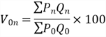
When we select only one commodity for studying, the simple price index for a given period is the percentage of the commodity price in the period to the price in the base period. The simple index calculation lays the foundations for understanding aggregate index constructions. The computation of the simple quantity index and the simple value index is similar to the simple price index. Here are three formulas to calculate the three types of index numbers:


where ![]() ,
, ![]() , and
, and ![]() are the price, quantity, and value in the base period, respectively;
are the price, quantity, and value in the base period, respectively; ![]() ,
, ![]() , and
, and ![]() are the price, quantity, and value in the given period (or the current period), respectively; and
are the price, quantity, and value in the given period (or the current period), respectively; and ![]() ,
, ![]() , and
, and ![]() are the simple price index, the simple quantity index, and the simple value index for the given period (or the current period), respectively.
are the simple price index, the simple quantity index, and the simple value index for the given period (or the current period), respectively.
Assume that a manufacturer produced one product only. Table 1 shows sales data for the past five years. We select 2015 as the base year; we then construct index numbers for prices, quantities, and sales values listed in the table.

Table 1 Sales Data for the Past Five Years (2015-2019)
1.1 Simple Price Indexes
According to Table 1, the price in the base year is 50, i.e., ![]() . Using the table’s data to substitute prices in the simple price index formula, we calculate and interpret the simple price index numbers, as illustrated in Table 2. We can use these index numbers to compare the commodity prices at different periods. The index numbers make comparison easy.
. Using the table’s data to substitute prices in the simple price index formula, we calculate and interpret the simple price index numbers, as illustrated in Table 2. We can use these index numbers to compare the commodity prices at different periods. The index numbers make comparison easy.

Table 2 The Constructions of Simple Price Index Numbers
We computed the simple index numbers by hand. We then use the R function “index.number.serie()” in the package “IndexNumber” (Saavedra-Nieves, 2020) to verify the manual calculations. The following R commands compute the simple price index numbers in the R console window. The function returns a list of index numbers, which agree with the manual calculations. If we set the arguments “opt.plot” and “opt.summary” to TRUE, the function plots a graphical description and prints the statistical summary of these numbers.
> library(IndexNumber)
> prices<-c(50,52,56,60,64)
> index.number.serie(prices,name="Price", opt.plot=FALSE, opt.summary=FALSE)
  Stages Price Index number
1      0    50          100
2      1    52          104
3      2    56          112
4      3    60          120
5      4    64          128
>
1.2 Simple Quantity Indexes and Value Indexes
From Table 1, the quantity and value in the base are 200 and 10,000, respectively. The construction of a simple quantity index or a simple value index is similar to that of the simple price index. Table 3 shows these two types of simple indexes. The index numbers provide a simple way of comparing numbers over periods. It often makes sense to use index numbers for displaying time-series data.

Table 3 The Constructions of Quantity and Value Index Numbers
We can continue to use the R function to verify the manual calculations. The following R commands compute the simple quantity index numbers and the simple value index numbers through the R console window. The outputs agree with the manual computations. It is advantageous to calculate index numbers by hand because the manual computations help us understand the construction methods.
> library(IndexNumber)
> quantities<-c(200,240,220,300,320)
> values<-c(10000,12480,12320,18000,20480)
> index.number.serie(quantities,name="Quantity")
  Stages Quantity Index number
1      0      200          100
2      1      240          120
3      2      220          110
4      3      300          150
5      4      320          160
> index.number.serie(values,name="Value")
  Stages Value Index number
1      0 10000        100.0
2      1 12480        124.8
3      2 12320        123.2
4      3 18000        180.0
5      4 20480        204.8
>
2 – Constructing Aggregate Indexes
When studying a basket of commodities (i.e., a group of related variables), we often find that the price changes are not uniform, as illustrated in Table 4. The percentage changes in the price vary from commodity to commodity. We cannot easily express changes in the general price level by using the percentage change in every commodity, especially when the number of commodities is enormous. However, we can use an aggregate price index (a single measure) to represent these changes. An aggregate index measures changes in the magnitude of a group of related variables over a period or regarding other characteristics, such as profession.
In this section, we construct price index numbers to illustrate the principles of constructing an aggregate index number. We can apply these principles to other fields. We explore two construction methods: the simple aggregative method and the weighted aggregative method. According to different weighting techniques, we further classify the weighted aggregative method into these three well-known methods: the Laspeyres method, the Paasche method, and the Fisher method.

Table 4 Sample Sales Data in Year 2011 and 2016 (Gupta, 2020)
2.1 Simple Aggregative Method
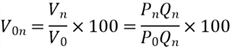
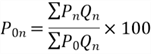
When neglecting each commodity’s relative importance to the general price level, we can use the simple aggregative method to construct a simple aggregate price index. To find the price index of a given year, we compute the sum of the prices in the given year. Next, we compute the sum of prices in the base year. The simple aggregate price index is the percentage of the first sum to the second sum. The index obtained from this method is also called the Dutot index. The formula for this method is as follows:
Using the data from Table 4 to substitute prices in the formula, we can obtain the simple aggregative price index, denoted by p01. We say the price has risen by 21.4%. In the context, ![]() stands for the price index for the period next to the base period.
stands for the price index for the period next to the base period. ![]() stands for the price index for the period second next to the base period and so on.
stands for the price index for the period second next to the base period and so on.
The function aggregated.index.number(), provided in the package “IndexNumber,” computes the simple aggregate price index. The function determines index numbers without weights for those in which there is more than one commodity (Saavedra-Nieves, 2020). To use the function, we create a matrix such that each column contains a commodity price, and each row contains the basket of commodities in a period. The following R console output shows the use of this function. The console output agrees with the manual calculation.
> library(IndexNumber)
> prices<-matrix(c(10,8,6,4,12,10,6,6), nrow=2, byrow = TRUE)
> aggregated.index.number(prices,"serie","BDutot","Price",opt.plot=FALSE,opt.summary=FALSE)
 Aggregate index number
Bradstreet-Dutot
  Stages Price 1 Price 2 Price 3 Price 4 Agg. index number
1      0      10       8       6       4          100.0000
2      1      12      10       6       6          121.4286
>
2.2 Weighted Aggregative Method
The quantity of commodities sold varies from commodity to commodity in the market. The units of measurement of prices may differ from each other as well. Therefore, each commodity may differently impact the general price level. When the index numbers do not appear to represent the price level, we can assign proper weights to the commodities according to their relative importance. However, determining the commodity weights according to their relative importance is a practical difficulty in constructing index numbers. We likely determine the weights arbitrarily and therefore bring biases to the index numbers.
In practice, we can determine the importance of a commodity’s price to the general price level by its quantities produced, consumed, or purchased; therefore, we generally use quantities as weights to construct weighted aggregative price indexes. Since the quantities in the base period are different from the quantities in the given period, as shown in Table 4, we have several ways to select quantity weights. We can choose one of these three construction methods: Laspeyres Method, Paasche Method, and Fisher Method.
2.2.1 Laspeyres Method
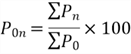
The Laspeyres method is the most frequently used in constructing weighted aggregate indexes (Hummelbrunner et al., 2003). This method considers the relative importance of each commodity and uses the base period quantities as the weights. Assume that we have a basket of commodities purchased in the base period, and the expense of these commodities is 100. The price index (the Laspeyres price index) for a given period provides an estimate of the expense of the same basket of commodities in the given period. We can use the following formula to calculate the weighted aggregate price index for the given period:

Using the data from Table 4 to substitute prices and quantities in the formula, we can obtain the Laspeyres price index, which uses the base period quantities as weights. According to the index number, the price level increased by 19.0%.

We can use the function laspeyres.index.number() to compute the weighted aggregate price index. The function determines index numbers with weights for several commodities (Saavedra-Nieves, 2020). To use the function, we create a matrix that each column contains a commodity price, and each row contains a group of commodities in a period. We also need to create a weight matrix in which the first row must contain weights. The following R console output shows the use of this function. The console output agrees with the manual calculation.
> library(IndexNumber)
> prices<-matrix(c(10,8,6,4,12,10,6,6), nrow=2, byrow = TRUE)
> weights<-matrix(c(30,15,20,10), nrow=1, byrow = TRUE)
> laspeyres.index.number(prices,weights,"Price",opt.plot=FALSE,opt.summary=FALSE)
Laspeyres index number
  Stages Price 1 Price 2 Price 3 Price 4 Agg. index number
1      0      10       8       6       4          100.0000
2      1      12      10       6       6          118.9655
>
For completeness, we provide formulas to calculate a weighted aggregate quantity index and weighted aggregate value index (Hummelbrunner et al., 2003). Gupta provides examples of calculation of these index numbers in his lecture (Gupta, 2020). When computing the weighted aggregate quantity index, we use the base period price as the weight. The weighted aggregate value index calculation takes into account the price and quantities of both the base period and the given period (or current period). All three formulas have the same denominator. It is worth noting that the weighted aggregate index numbers measure only overall change in a group of related variables and indicate only broad trends. They do not provide accurate information for any individual variable.
2.2.2 Paasche Method
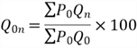
When computing an aggregate price index, quantities in the given period usually differ from quantities in the base period. The Paasche method takes the given period quantities as weights and obtains Paasche price index numbers. Assuming that we have a basket of commodities purchased in a given period and that the expenditure on the same commodities is 100 in the base period, the Paasche price index indicates the estimation of these commodities’ expense in the given period. For the sake of easy understanding, we can say a Paasche index estimates the cost of today’s basket at yesterday’s prices. The following formula can calculate Paasche price index numbers:
Substituting prices and quantities of the formula using data in Table 4, we obtain the Paasche price index. This method takes the given period quantities as weights and shows that the price level has increased by 19.8%.

The function paasche.index.number() can be used to compute the weighted aggregate price index using the Paasche method. The function determines index numbers with weights for a basket of commodities (Saavedra-Nieves, 2020). To use the function, we create a matrix that each column contains a commodity price, and each row contains a group of commodities in a period. We also need to create a weight matrix in which the last row should contain weights. The following R console output shows the use of this function. The console output agrees with the manual calculation.
> library(optimbase)
> library(IndexNumber)
> prices<-matrix(c(10,8,6,4,12,10,6,6), nrow=2, byrow = TRUE)
> weights<-rbind(ones(1,4),c(50,25,30,20)) # Weights at the last row
> paasche.index.number(prices,weights,"Price",opt.plot=FALSE,opt.summary=FALSE)
Paasche index number
  Stages Price 1 Price 2 Price 3 Price 4 Agg. index number
1      0      10       8       6       4          100.0000
2      1      12      10       6       6          119.7917
>
2.2.3 Fisher Method
While the Laspeyres price index uses the base period quantities as weights, and the Paasche takes the given period quantities as weights, the Fisher method calculates the geometric mean of the Laspeyres index and the Paasche index. Therefore, the Fisher method considers the price and quantities of both the base period and the given period (or the current period). Thus, we often consider the Fisher method to be an ideal method. We can use the following formula to calculate the Fisher price index:

For the sake of simplicity, we use the index numbers calculated in Sections 2.2.1 and 2.2.2 to substitute the Laspeyres index and the Paasche Index in the formula; we then obtain the Fisher price index. The index number reveals that the price level increased by 19.4%.
We continue to use a function in the “IndexNumber” package to compute the weighted aggregate price index. The function fisher.index.number() determines index numbers with weights for those in which several commodities exist (Saavedra-Nieves, 2020). To use this function, we create a matrix in which each column contains a commodity price, and each row contains a group of commodities in a period. We also need to create a weight matrix in which each column contains a commodity quantity (weight), and each row contains a group of commodities in a period. The following R console output shows the use of this function. The console output agrees with the manual calculation.
> library(IndexNumber)
> prices<-matrix(c(10,8,6,4,12,10,6,6), nrow=2, byrow = TRUE)
> weights<-matrix(c(50,25,30,20,30,15,20,10), nrow=2, byrow = TRUE)
> fisher.index.number(prices,weights,"Price",opt.plot=FALSE,opt.summary=FALSE)
Laspeyres index number
Paasche index number
Fisher index number
  Stages Price 1 Price 2 Price 3 Price 4 Agg. index number
1      0      10       8       6       4          100.0000
2      1      12      10       6       6          119.3779
>
Summary
In this article, we introduced the concept of index numbers with examples. We then explored the formulas to calculate the simple price index, the simple quantity index, and the simple value index. The R function, index.number.serie(), checked the manual calculations.
We demonstrated the aggregate index and its constructing methods in the subsequent sections. We went through the Laspeyres method, the Paasche method, and the Fisher method with examples. We also use other R functions to verify the manual calculation.
It is essential to understand that each index employs a distinguished constructing method based on data availability, degree of accuracy, and the studying purpose. We also recognized that the index construction process is challenging. Index numbers are good for immediate assessments, but we cannot solely rely on them for making decisions.
Reference
Baldoni, E. (2017). multilaterals: Transitive Index Numbers for Cross-Sections and Panel Data. https://cran.r-project.org/web/packages/multilaterals/index.html.
Dakpo, K., Desjeux, Y., & Latruffe, L. (2018). productivity: Indices of Productivity Using Data Envelopment Analysis (DEA). https://cran.r-project.org/web/packages/productivity/index.html.
Duffin, E. (2020). Average Canadian undergraduate tuition fees 2006-2020. https://www.statista.com/statistics/542989/canadian-undergraduate-tuition-fees/.
Gupta, P. (2020). Class 11: Statistics | Index Numbers – Conclusion. https://youtu.be/AEbrq8FW8XA.
Giraud, A. (2020). How to build a powerful business index? https://towardsdatascience.com/how-to-build-an-index-452f5018d5aa.
Henningsen, A. (2017). micEconIndex: Price and Quantity Indices. https://cran.r-project.org/web/packages/micEconIndex/index.html.
Hummelbrunner, S. A., Rak, L. J., Fortura, P., & Taylor, P. (2003). Contemporary Business Statistics with Canadian Applications (3rd Edition). Prentice Hall.
MBN. (2019). What is an index number? Definition and meaning. https://marketbusinessnews.com/financial-glossary/index-number-definition-meaning/.
Saavedra-Nieves, A., & Saavedra-Nieves, P. (2020). IndexNumber: Index Numbers in Social Sciences. https://cran.r-project.org/web/packages/IndexNumber/index.html.
Smith, B. (2018). Ultimate Performance Index Guide. https://madetomeasurekpis.com/blog/2018/10/21/ultimate-performance-index-guide/.
White, G. (2020). IndexNumR: A Package for Index Number Calculation. https://cran.r-project.org/web/packages/IndexNumR/vignettes/indexnumr.html.
Next Steps
- The author skipped some essential topics about index numbers, such as characteristics, limitations, and adequacy tests. Moreover, the article did not explore a step-by-step process of constructing an index. Nevertheless, this article introduced index number basics and laid the foundation for studying index numbers in depth. To know how to build an index, we recommend Giraud’s article, How to build a powerful business index. Furthermore, Smith’s article, Ultimate Performance Index Guide, is also worth reading. Index numbers are useful in almost all fields, and they are critical in the economic and business fields. Before adopting the index number technique in our projects, we should be aware that the technique has certain limitations. These limitations have significantly reduced the usefulness of the technique. The article used the “IndexNumber” package. Several other packages also provided the related functionalities. These packages include IndexNumR (White, 2020), micEconIndex (Henningsen, 2017), multilaterals (Baldoni, 2017), and productivity (Dakpo et al., 2018). It is worth being aware of these packages. The sample data in Table 4 was quoted from https://youtu.be/AEbrq8FW8XA. The video clip also includes the computation of weighted aggregate quantity indexes and the weighted aggregate value index.
- Check out these related tips:

Nai Biao Zhou has twenty years of experience in software development, with strong analytical skills and a broad range of computer expertise.
He has fifteen years of experience in development and maintenance of database applications on SQL Server in OLTP/OLAP/BI environments.
He has a master’s degree in Control Engineering and is pursuing a Master of Science degree in Predictive Analytics.
Knowledge/Skills
Advanced computer programming skills and well versed with C/C#, Java, ASP.NET, JavaScript, and SQL.
In depth knowledge of Solution Architecture, and Software Development Life Cycle (SDLC).
Microsoft Certified Application Developer (MCAD) since 2004.
- MSSQLTips Awards: Author of the Year – 2021 | Rising Star (50+ tips) – 2024 | Author Contender – 2020, 2023
Appreciate