Perform Statistical Calculations on SQL Server Data

By: Rick Dobson | Updated: 2023-08-10 | Comments (4) | Related: > TSQL

Problem

I was recently assigned to be the T-SQL developer within our firm's newly formed analytics team. SQL Server is our system of record, and the team needs a T-SQL professional to extract, transform, query, and perform preliminary statistical analyses of content stored in databases stored on our SQL Server instances. I recall reading an introductory presentation on the T-SQL Starter Statistics Package. Please present some additional examples for the package that can help to prepare me for statistical analysis projects.

Solution

The T-SQL Starter Statistics Package consists of a series of stored procedures. Each stored procedure is for a different type of statistical technique. To use the stored procedures in the package, you can populate a temporary table with rows from a query. Then, invoke a stored procedure to generate the desired output.

The original tip for the T-SQL Starter Statistics Package uses cross-sectional data. This tip focuses on examples with time series data. Also, the original tip provides some background on each statistical analysis technique before invoking the stored procedure for the technique. This tip merely names the technique and then illustrates how to load the data into a temp table for processing by a stored procedure. The results set from each stored procedure invocation is presented and described to help you understand each example. One example in this tip highlights how to download data as a CSV file from an internet source into a temp table for additional processing. Depending on your project requirements, you can optionally save the downloaded data within SQL Server for future reference.

If you could benefit from a brief review of temp tables, please refer to this prior tip and its related tips. The full collection of tips on temp tables will be more than sufficient to equip you to handle the examples in this tip.

A Stored Procedure for the Median of a Single Category of Items

The median is a measure of central tendency. You can think of the median as the value that divides an ordered set of numbers from within a dataset into top and bottom halves. This value corresponds to the fiftieth percentile of the ordered values in a dataset.

The T-SQL percentile_cont function can find a value corresponding to any given percentile for an ordered set of values in a column of a results set or table. If you specify .5 as the input parameter for the function, then the function returns the median value for the source dataset.

The following script creates a fresh copy of the compute_overall_median stored procedure in the DataScience database. You can use any other database you prefer; just change the argument for the Use statement at the top of the script for the alternate database.

The script inside the stored procedure contains two select statements and a return statement. The inner select statement generates a results set for processing by the outer select statement.
The outer select statement in the stored procedure shows the syntax for the percentile_cont function
- The use of the distinct keyword returns a single median value for the column_for_median column values in the ##table_for_overall_median table
- The .5 value inside the function designates the return of the fiftieth percentile
- The within group clause designates a column of values within the ##table_for_overall_median table on which to compute a median
- The over clause is required by the percentile_cont function syntax. However, the partition argument does not segment the source data into separate groups of rows because all rows have the same category_value column value (namely, overall)
The inner select statement is for a derived table based on the ##table_for_overall_median table
The return statement passes back control to the script invoking the compute_overall_median stored procedure
The final go keyword instructs SQL Server to end the batch creating the stored procedure. This keyword is only required when there are additional batches in the SQL script file for subsequent processing steps

Use DataScience
go
 
-- drop any prior version of the dbo.compute_overall_median  stored procedure
drop procedure if exists dbo.compute_overall_median
go
 
create procedure dbo.compute_overall_median
as
begin
   set nocount on;
 
   -- distinct in select statement shows just one overall median row value
   select 
      distinct percentile_cont(.5) 
         within group (order by column_for_median) 
         over(partition by category_value)
   from
   (
      select 
          * 
         ,'overall' category_value 
      from ##table_for_overall_median
   ) for_median
 
   return
 
end
go

The next script manages the use of the compute_overall_median stored proc.

The script begins by populating a fresh version of the ##table_for_overall_median table based on the symbol_date table
The symbol_date table contains price values for ticker symbols by date. This table is just like any other time series dataset, such as sales by date for salespersons or products manufactured by date from different plants
This portion of the script extracts just rows from the symbol_date table with symbol value of QQQ. There are five other symbols in the symbol_date table, but none of these other symbol values are accepted by the where clause criterion in the initial select statement
Next, the script displays the rows of the ##table_for_overall_median table
Finally, the script invokes the compute_overall_median stored procedure and retrieves the returned value from the stored procedure via the @tmpTable table variable. The script ends with a select statement that displays the value in the table variable

use DataScience
go
 
-- populate ##table_for_overall_median
-- based on symbol_date
 
-- drop any prior version of the table
drop table if exists ##table_for_overall_median
 
-- insert query result set into global temp table
-- based on symbol_date table
-- assign column_for_median as alias for target column
select symbol, date, [close] [column_for_median]
into ##table_for_overall_median
from symbol_date
where symbol = 'QQQ'
 
-- display rows in ##table_for_overall_median
select * from ##table_for_overall_median
 
-- invoke compute_overall_median stored procedure
-- display median as median_value from @tmpTable
declare @tmpTable table (median_value real)
insert into @tmpTable
exec dbo.compute_overall_median
select * from @tmpTable

Here is the output from the preceding script:

The top pane in the Results tab shows the first eleven rows from the ##table_for_overall_median table
The bottom pane shows the median for all column_for_median row values
Notice that all the rows are for the QQQ ticker
From the bottom right border of the screenshot, you can tell there are 5972 rows in the ##table_for_overall_median table. The median value of 63.17375 in the bottom pane is the 5973^rd row in the Results tab

Stored Procedure for the Median of a Single Category of Items

A Stored Procedure for the Medians of a Group of Categories

The preceding section computes and displays the median for a single category of items. The single category of items is priced for the QQQ ticker symbol. If you need medians for multiple different tickers from a time series table like the symbol_date table, you can repeatedly execute the compute_overall_median stored procedure for each of the distinct symbols in the symbol_date table. However, there is a more efficient way to return the medians for each ticker symbol. In short, you can use the partition setting within the percentile_cont function.

The following script shows a modified version of the stored procedure from the preceding section. The version for this section has the name compute_median_by_category instead of compute_overall_median. The category in this example is the ticker symbol for a row. The compute_median_by_category stored procedure returns a distinct median value for each distinct ticker symbol. To achieve this goal, the ##table_for_median_by_category table needs to be populated with rows having two or more distinct symbols.

Here is the script for the new stored procedure. It is similar to the stored procedure in the preceding section. The most important difference is the from clause for the outer select statement. The inner select statement expects two select list items named category and column_for_median. The value of the category column values is derived from the source data in the ##table_for_median_by_category table instead of the ##table_for_overall_median table (as in the preceding section).

use DataScience
go
 
-- drop any prior version of the compute_median_by_category procedure
drop procedure if exists compute_median_by_category
go
 
create procedure compute_median_by_category
as
begin
   set nocount on;
 
   select 
      *
   from
   (
      -- compute median by gc_dc_symbol
      -- distinct in select statement shows just one median per symbol
      select 
         distinct category
        ,percentile_cont(.5) 
            within group (order by column_for_median) 
            over(partition by category) median_by_category
      from
      (
         select 
            category
           ,column_for_median 
         from ##table_for_median_by_category
      ) for_median_by_category
   ) for_median_by_category
   order by category
 
   return
 
end
go

The following script is for invoking the compute_median_by_category stored procedure and displaying its results set. The script starts by populating the ##table_for_median_by_category table from the symbol_date table. For the example in this section, there is no where clause in the script for populating the global temp table (##table_for_median_by_category). This permits all the ticker symbols in the symbol_date table to be passed to the ##table_for_median_by_category table. Recall that in the preceding section just one symbol was passed to the ##table_for_overall_median table; this symbol had a value of QQQ. The rest of the second script segment for this section is identical in function to the second script section in the preceding segment.

-- populate ##table_for_overall_median
-- based on symbol_date
 
-- drop any prior version of the table
drop table if exists ##table_for_median_by_category
 
-- insert query result set into global temp table
-- based on symbol_date table
-- assign column_for_median as alias for target column
-- also assign category as alias for column with category values (symbol)
select symbol [category], date, [close] [column_for_median]
into ##table_for_median_by_category
from symbol_date
 
 
-- display ##table_for_median_by_category
select *
from ##table_for_median_by_category
order by category, date
 
-- invoke compute_median_by_category stored procedure
-- display category and median_by_category from @tmpTable
declare @tmpTable TABLE (category varchar(5), median_by_category real)
 
insert into @tmpTable
exec compute_median_by_category
 
-- display medians by category
select * from @tmpTable

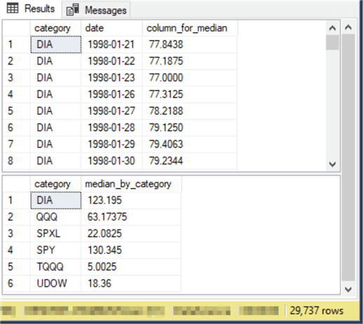
Here is the output from the preceding script:

The top pane in the Results tab shows the first eight rows from the ##table_for_median_by_category table. These rows are all for the first ticker symbol (DIA) in alphabetical order within the table. Other rows in the table may have different ticker symbols (QQQ, SPXL, SPY, TQQQ, and UDOW)
The bottom pane in the Results tab shows the median for each of the ticker symbols in the ##table_for_median_by_category table

A Stored Procedure for the Medians of a Group of Categories

Downloading Historical Index Values from the Wall Street Journal

A couple of prior tips ("SQL Server Data Mining for Leveraged Versus Unleveraged ETFs as a Long-Term Investment" and "Adding a Buy-Sell Model to a Buy-and-Hold Model with T-SQL") examined the symbol_date table. When analyzing a dataset, it is not unusual to discover a need for additional related kinds of data. The symbol_date table contains time series prices for six ETF ticker symbols based on major market indexes. These ETF prices were collected from Yahoo Finance in the first of the prior tips. The six ETFs are based on three major market indexes (the Dow Jones Industrial Average, the S&P 500 index, and the Nasdaq 100 index); one set of three tickers is for unleveraged ETFs, and the other set of ETFs is for leveraged ETFs. The unleveraged ETFs are designed so that there should be a nearly perfect linear correlation between the unleveraged ETFs and their underlying index.

No prior tip in MSSQLTips.com examined the underlying indexes for the unleveraged ETFs. This section in the current tip demonstrates how to collect historical values for the three major market indexes. This kind of data is available from multiple sources for free. In this section, the Wall Street Journal website (wsj.com) is used as a resource for collecting historical major market index values.

The tickers for the major market indexes on the Wall Street Journal website are as follows:

DJI for the Dow Jones Industrial Average
NDX for the Nasdaq 100 Index
SPX for the S&P 500 index

Security ticker symbols can change from one source to another. Therefore, you should always verify the ticker symbols for the securities you want to examine whenever you are working with a new site.

You can navigate your browser to the page for an index by entering the URL for an index in the address box of your browser. The URL hyperlink column in the following table displays the name of the URL that you can enter into your browser for navigating to a web page for an index. Also, clicking a hyperlink in the following table will open your browser to the page for downloading index values.

Specify on the web page start and end dates for values you seek to download
Click the download a spreadsheet link on the web page to copy the specified data to your Windows download folder

Major Market Index Name	Ticker Symbol	URL hyperlink
Dow Jones Industrial Average	DJI	https://www.wsj.com/market-data/quotes/index/DJI/historical-prices
Nasdaq 100 Index	NDX	https://www.wsj.com/market-data/quotes/index/NDX/historical-prices
S&P 500 Index	SPX	https://www.wsj.com/market-data/quotes/index/SPX/historical-prices

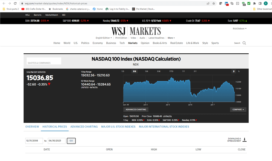
The following screenshot is a slightly edited version of the Wall Street Journal web page for downloading Nasdaq 100 index values. The editing is to specify start and end dates of downloaded data from 2008-12-31 through 2023-06-30.

Clicking the GO button after entering the start and end dates prepares the data for downloading
After the data is prepared, click the Download a spreadsheet link on the right edge of the screen opposite the GO button. This copies the selected range of time series values for the NDX ticker to your Windows download folder
The copied file will have the name HistoricalPrices.csv. You should rename the file if you are working with more than one ticker symbol in a single browser session. In the example for this tip, the downloaded file is named NDX.csv. You can assign corresponding file names for the S&P 500 index (SPX.csv) and the Dow Jones Industrial Average (DJI.csv)
A good practice is to copy the downloaded files from the Windows download folder to a more dedicated storage location for the three index files

Downloading Historical Index Values from the Wall Street Journal

After downloading and relocating the CSV files for the tickers you are processing, you can import the CSV files into SQL Server tables. The following script shows one approach for accomplishing this goal.

First, the script creates fresh copies of the #temp_ohlc_values_for_indexes and #temp_ohlc_values_for_indexes_with_symbol tables
- The #temp_ohlc_values_for_indexes table stores the index values for a ticker as downloaded from the source website. Recall that these values do not include a ticker symbol
- The #temp_ohlc_values_for_indexes_with_symbol table adds a column for the symbol for the ticker values in a downloaded set of values for a ticker, such as NDX for the Nasdaq 100 index values
Next, the script copies the values from a file with index values for each of the three tickers, in turn, starting with the SPX ticker and continuing through the NDX and DJI tickers
- The first step for each ticker is to transfer the downloaded data for a ticker to the #temp_ohlc_values_for_indexes table; the #temp_ohlc_values_for_indexes table temporarily holds the index values for the current ticker being processed
- The second step is to populate a symbol column with the value of the current ticker being processed and then add the symbol column to the columns of index values imported into the #temp_ohlc_values_for_indexes table; the outcome of this step is to update the #temp_ohlc_values_for_indexes_with_symbol table with the symbol and index columns for the current ticker being processed
- The third step truncates the values in the #temp_ohlc_values_for_indexes table. Then, this table is re-populated with index values for a new ticker symbol if one remains to be processed
- At the end of these steps, the #temp_ohlc_values_for_indexes_with_symbol table is updated with index values for however many tickers you are processing. For the example in this tip, these are the three tickers for major market indexes

-- create temp tables for indexes
 
-- this table is for storing index values from WSJ source
drop table if exists #temp_ohlc_values_for_indexes
 
create table #temp_ohlc_values_for_indexes(
 date date
,[open] dec(19,4)
,high dec(19,4)
,low dec(19,4)
,[close] dec(19,4)
)
go
 
-- this table is for adding index name as symbol
drop table if exists #temp_ohlc_values_for_indexes_with_symbol
 
create table #temp_ohlc_values_for_indexes_with_symbol(
 symbol nvarchar(10)
,date date
,[open] dec(19,4)
,high dec(19,4)
,low dec(19,4)
,[close] dec(19,4)
)
 
---------------------------------------------------------
 
-- next, do a bulk insert
bulk insert #temp_ohlc_values_for_indexes
from 'C:\DataScienceSamples\ETF_Comps\SPX.csv'
with (
   FIELDTERMINATOR = ',', 
   FIRSTROW = 2,
   ROWTERMINATOR = '0x0a'
);
 
-- populate symbol column in #temp_ohlc_values_for_indexes_with_symbol
-- assign ^GSPC to @symbol
declare @symbol nvarchar(10) = 'SPX'
 
-- populate symbol column in #temp_ohlc_values_for_indexes_with_symbol
-- with @symbol value
insert into #temp_ohlc_values_for_indexes_with_symbol
select @symbol symbol, *
from
(
select * from #temp_ohlc_values_for_indexes
) index_value_without_symbol
 
---------------------------------------------------------
 
-- empty #temp_ohlc_values_for_indexes
truncate table #temp_ohlc_values_for_indexes
 
-- next, do a bulk insert
bulk insert #temp_ohlc_values_for_indexes
from 'C:\DataScienceSamples\ETF_Comps\NDX.csv'
with (
   FIELDTERMINATOR = ',', 
   FIRSTROW = 2,
   ROWTERMINATOR = '0x0a'
);
 
-- populate symbol column in #temp_ohlc_values_for_indexes_with_symbol
-- assign ^NDX to @symbol
set @symbol = 'NDX'
 
-- populate symbol column in #temp_ohlc_values_for_indexes_with_symbol
-- with @symbol value
insert into #temp_ohlc_values_for_indexes_with_symbol
select @symbol symbol, *
from
(
select * from #temp_ohlc_values_for_indexes
) index_value_without_symbol
 
---------------------------------------------------------
 
truncate table #temp_ohlc_values_for_indexes
 
-- next, do a bulk insert
bulk insert #temp_ohlc_values_for_indexes
from 'C:\DataScienceSamples\ETF_Comps\DJI.csv'
with (
   FIELDTERMINATOR = ',', 
   FIRSTROW = 2,
   ROWTERMINATOR = '0x0a'
);
 
-- populate symbol column in #temp_ohlc_values_for_indexes_with_symbol
-- assign DJI to @symbol
set @symbol  = 'DJI'
 
-- populate symbol column in #temp_ohlc_values_for_indexes_with_symbol
-- with @symbol value
insert into #temp_ohlc_values_for_indexes_with_symbol
select @symbol symbol, *
from
(
select * from #temp_ohlc_values_for_indexes
) index_value_without_symbol
 
-- display contents of #temp_ohlc_values_for_indexes_with_symbol
-- for all three indexes
select * 
from #temp_ohlc_values_for_indexes_with_symbol
order by symbol asc, date desc

The following screenshot shows the first eight rows from the select statement at the end of the preceding script. All of these values are for the DJI ticker symbol. Therefore, they are Dow Jones Industrial Average values.

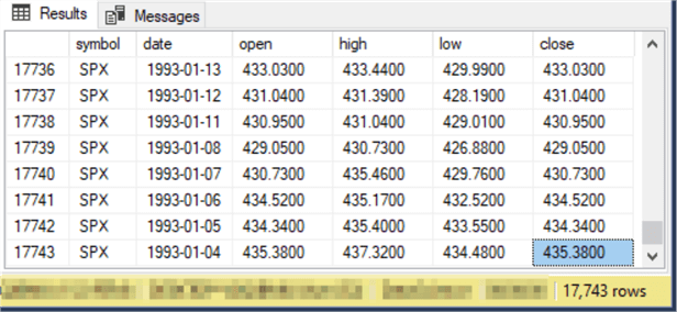
The next screen is for the last eight rows from the #temp_ohlc_values_for_indexes_with_symbol table displayed by the final select statement in the preceding script. All these rows are for the SPX ticker, representing the S&P 500 index.

The rows for the NDX ticker are in the #temp_ohlc_values_for_indexes_with_symbol table between the rows for the DJI ticker and the SPX ticker. As you can see from the bottom border of the following and preceding screenshots, there are 17743 rows in the #temp_ohlc_values_for_indexes_with_symbol table.

Correlating Major Market ETF Price Values with Underlying Index Values

One important reason for wanting historical index values is to verify the nature of their relationship to ETF securities. For example, we can ask

Are ETF prices in a perfect linear relationship with their underlying index?
Is the relationship between a major market underlying index for an ETF obviously different than for any alternate major market index?

The first step to answering these questions is to create datasets with ETFs and their underlying index, as well as between ETFs and an alternate major market index.

The second step is to apply a statistical tool that assesses the strength of the linear relationship between two sets of values, such as ETF closing prices and major market index closing prices.

You might be wondering: why not just compare different major market underlying indexes directly to one another? There are several answers to this question.

First, you cannot invest directly in major market indexes. This is because major market indexes are not tradeable securities. In other words, you cannot buy and sell major market indexes. This is because they are not a financial security but rather an average of the financial securities in an index. Furthermore, the number of component securities is not the same across all major market indexes. In addition, the component securities in an index can change over time
Second, ETFs based on major market indexes are available for traders to buy and sell. There is not just one ETF per index. Different businesses can sponsor different ETFs for the same underlying index. This tip tracks the earliest ETF for each of three major market indexes examined in this tip
- The DIA (also known as the SPDR Dow Jones Industrial Average ETF Trust) is for the Dow Industrial Average; it was initially offered for sale in January 1998
- The SPY (also known as the SPDR S&P 500 ETF Trust) is for the S&P 500 index; it was initially offered for sale in January 1993
- The QQQ (also known as the Invesco QQQ Trust) is for the Nasdaq 100 index; it was initially offered for sale in March 1999
It is also relevant that major market indexes typically have longer historical records than the ETFs based on them. Therefore, if you seek extensive historical data to verify models for buying and selling securities, indexes may be preferable to ETFs

The coefficient of determination is an indicator of the goodness of fit of a predicted set of values (y values) to an observed set of values (x values). This tip deals with x and y values in a linear regression format with a correlation coefficient or r and a coefficient of determination that equals r². The following script is more fully discussed in the "A stored procedure to compute coefficients of determination" section of the T-SQL Starter Statistics Package tip.

You can change the database for storing the stored procedure to any other one you prefer instead of DataScience
The compute_coefficient_of_determination stored procedure depends on an external data source named ##temp_xy. This data source contains the x value set and the y value set. You must specify the contents of the external data source before invoking the compute_coefficient_of_determination stored procedure

use DataScience
go
 
drop procedure if exists dbo.compute_coefficient_of_determination
go
 
create procedure compute_coefficient_of_determination 
as 
  begin 
      set nocount on; 
      -- compute coefficient of determination 
      -- based on correlation coefficient 
      select 
         sum(y_minus_mean_sq) sum_of_y_sq_devs, 
         sum(x_minus_mean_sq) sum_of_x_sq_devs, 
         sum(x_y_mean_product) sum_of_xy_product_devs, 
         sum(x_y_mean_product) / ( sqrt(sum(y_minus_mean_sq)) * sqrt(sum(x_minus_mean_sq)) ) correlation_coefficient, 
         power(sum(x_y_mean_product) / ( sqrt(sum(y_minus_mean_sq)) * sqrt(sum(x_minus_mean_sq)) ), 2) coefficient_of_determination 
      from   
      ( 
         -- compute power deviations from mean 
         select 
            x, 
            y, 
            ( x - avg_x )                 x_minus_mean, 
            power(( x - avg_x ), 2)       x_minus_mean_sq, 
            ( y - avg_y )                 y_minus_mean, 
            power(( y - avg_y ), 2)       y_minus_mean_sq, 
            ( x - avg_x ) * ( y - avg_y ) x_y_mean_product 
         from  
         ( 
            -- inputs for coefficient of determination 
            select * 
            from (select cast(x as float) x, cast(y as float)  y from ##temp_xy) source_data 
            cross join (select avg(cast(y as float)) avg_y from ##temp_xy) avg_y 
            cross join (select avg(cast(x as float)) avg_x from ##temp_xy) avg_x
         ) for_r_squared_inputs
      ) for_r_squared 
      return 
  end 
go

Here is a pair of scripts for invoking the compute_coefficient_of_determination stored procedure.

The first script performs a join between QQQ and NDX close values as the source data for the stored procedure. This script begins by creating the ##temp_xy table. Next, the QQQ close and the NDX close values are inserted into the ##temp_xy table. The first script ends by invoking the compute_coefficient_of_determination stored procedure for the values in the ##temp_xy table
The second script starts by truncating the ##temp_xy table. Then, the temp table is re-populated with the QQQ close and the SPX close values. The second script also ends by invoking the stored procedure
The output from these two scripts allows a comparison of the coefficient of determination between QQQ and NDX close values versus the coefficient of determination between QQQ and NDX close values

------------------------------------------------------------------------------------------
------------------------------------------------------------------------------------------
 
-- table with x and y values for coefficient of determination
 
drop table if exists ##temp_xy
 
create table ##temp_xy 
(
   x float,
   y float
)
go
 
-- populate ##temp_xy with ... NDX_close from for_NDX_close
-- and QQQ_close from for_QQQ_close
 
insert into ##temp_xy
select for_NDX_close.NDX_close,for_QQQ_close.QQQ_close
from
(
-- for QQQ close values
select 
 symbol
,date
,[close] [QQQ_close]
from DataScience.dbo.symbol_date
where symbol = 'QQQ'
) for_QQQ_close
 
join
 
(
-- values for ^NDX_close
select 
 symbol
,date 
,[close] [NDX_close]
from #temp_ohlc_values_for_indexes_with_symbol
where symbol = 'NDX'
) for_NDX_close
 
on for_QQQ_close.date = for_NDX_close.date
 
exec dbo.compute_coefficient_of_determination
 
-----------------------------------------------------------
 
truncate table ##temp_xy 
 
-- populate ##temp_xy with ... SPX_close from for_SPX_close
-- and QQQ_close from for_QQQ_close
 
insert into ##temp_xy
select for_SPX_close.SPX_close,for_QQQ_close.QQQ_close
from
(
-- for QQQ close values
select 
 symbol
,date
,[close] [QQQ_close]
from DataScience.dbo.symbol_date
where symbol = 'QQQ'
) for_QQQ_close
 
join
 
(
-- values for SPX_close
select 
 symbol
,date date
,[close] [SPX_close]
from #temp_ohlc_values_for_indexes_with_symbol
where symbol = 'SPX'
) for_SPX_close
 
on for_QQQ_close.date = for_SPX_close.date
 
exec dbo.compute_coefficient_of_determination

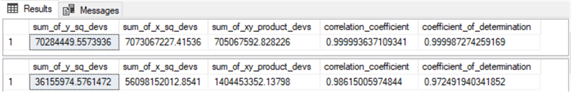
Here is the output from the preceding script segment.

The top pane assesses the correspondence between QQQ and NDX close values. The coefficient of determination is within .00001 of 1, where 1 denotes perfect correspondence.
The second pane assesses the correspondence between QQQ and SPX close values. This coefficient of determination is also excellent, but it is not quite as excellent as for QQQ and NDX close values.

Correlating Major Market ETF Price Values with Underlying Index Values

Here is another script segment to compare the strength of the correspondence between an ETF and its underlying major market index and an alternative major market index. The first pair is SPY and SPX, the underlying index for SPY. The second pair is for SPY and NDX, an alternative underlying index.

truncate table ##temp_xy
 
-- populate ##temp_xy with ... SPX_close from for_SPX_close
-- and SPY_close from for_SPY_close
 
insert into ##temp_xy
select for_SPX_close.SPX_close,for_SPY_close.SPY_close
from
(
-- for SPY close values
select 
 symbol
,date
,[close] [SPY_close]
from DataScience.dbo.symbol_date
where symbol = 'SPY'
) for_SPY_close
 
join
 
(
-- values for SPX_close
select 
 symbol
,date 
,[close] [SPX_close]
from #temp_ohlc_values_for_indexes_with_symbol
where symbol = 'SPX'
) for_SPX_close
 
on for_SPY_close.date = for_SPX_close.date
 
exec dbo.compute_coefficient_of_determination
 
-----------------------------------------------------------
 
truncate table ##temp_xy
 
-- populate ##temp_xy with ... NDX_close from for_NDX_close
-- and SPY_close from for_SPY_close
 
insert into ##temp_xy
select for_NDX_close.NDX_close,for_SPY_close.SPY_close
from
(
-- for SPY close values
select 
 symbol
,date
,[close] [SPY_close]
from DataScience.dbo.symbol_date
where symbol = 'SPY'
) for_SPY_close
 
join
 
(
-- values for NDX_close
select 
 symbol
,date 
,[close] [NDX_close]
from #temp_ohlc_values_for_indexes_with_symbol
where symbol = 'NDX'
) for_NDX_close
 
on for_SPY_close.date = for_NDX_close.date
 
exec dbo.compute_coefficient_of_determination

Here is the output from the preceding script.

The correspondence between the underlying index (SPX) for the SPY is not quite as strong as for the NDX underlying index and the QQQ. Nevertheless, the correspondence in terms of the coefficient of determination is still within .00002, which is still excellent
Also, the correspondence of the NDX, an alternative index, versus the SPY was weaker than for SPX index versus the SPY
For both sets of comparisons, the underlying index for a major market ETF gave a superior match than an alternate index for a major market ETF

Next Steps

There are four sections in this tip. Three sections focus on three different statistical analysis techniques. One section describes downloading and importing data from the internet to SQL Server. After reading this tip, the best way to truly learn the T-SQL code for implementing the statistical techniques is to try them with sample data from prior tips and the current tip. Once you duplicate the results in this tip, the next step is to use the techniques with your own data.

The first and second sections present two different use cases for computing medians with T-SQL in SQL Server. The first section shows how to compute a median for all the numbers in a dataset. The second section shows how to compute a median for each category of numbers in a dataset. The dataset for the first two sections is described and processed in a prior tip ("SQL Server Data Mining for Leveraged Versus Unleveraged ETFs as a Long-Term Investment"). You can retrieve the data for these two sections from that tip.

The third section demonstrates downloading CSV files from the Wall Street Journal website. Then, it shows how to read the CSV file into SQL Server temp tables. The downloaded and imported data complement the data from the "SQL Server Data Mining for Leveraged Versus Unleveraged ETFs as a Long-Term Investment" tip. The newly collected data in the third section serves as source data for the data in the first, second, and fourth sections. That is because the ETF security prices in the first, second, and fourth sections are based on indexes downloaded in the third section. The downloaded index CSV files are included in a download for this tip.

The fourth section illustrates how to use a stored procedure for computing the coefficient of determination between two different sets of numbers. One set of numbers is time series values with prices for two different securities. Another set of numbers are index values that serve as source data for the two sets of security prices. The coefficient of determination confirms which set of index values matches which set of security prices. This section confirms how easy it can be with T-SQL to verify the correspondence between two different sets of numbers.

About the author

Rick Dobson is an author and an individual trader. He is also a SQL Server professional with decades of T-SQL experience that includes authoring books, running a national seminar practice, working for businesses on finance and healthcare development projects, and serving as a regular contributor to MSSQLTips.com. He has been growing his Python skills for more than the past half decade -- especially for data visualization and ETL tasks with JSON and CSV files. His most recent professional passions include financial time series data and analyses, AI models, and statistics. He believes the proper application of these skills can help traders and investors to make more profitable decisions.

This author pledges the content of this article is based on professional experience and not AI generated.

View all my tips

Article Last Updated: 2023-08-10

Use T-SQL to Perform Statistical Calculations on SQL Server Data